Curriculum

Week 3. Optimizers and training regime

Phase 1. Foundations · week 3 of 24

Learn in the app: tutor, coding problems →

Core: SGD, momentum, Adam and bias correction, AdamW from scratch, warmup and clipping · Depth: parameter groups, inequalities and limit theorems (track D) · ≈ 10 h core / 20 h total

The gradient tells you where to go, and the optimizer decides how far. AdamW is used in almost every LLM, and its state together with the fp32 copy of the weights takes 12 of the 16 bytes per parameter (week 9), which is exactly what ZeRO shards first (week 14). Without warmup and clipping you cannot read the loss spikes in week 10.

Theory

• SGD: θ ← θ − ηg

In plain terms. A dataset has four examples with gradients 1, 3, 5, 7, and the full gradient is their mean, 4. A batch of one random example gives 1, 3, 5 or 7, and on average exactly 4: the estimate is noisy but unbiased (its mean equals the truth). A batch of two also gives 4 on average, but with less spread. The variance falls as 1/B and the standard deviation as 1/√B: a batch four times larger only halves the noise.

• Stochastic gradient: the gradient over a random mini-batch is an unbiased estimate of the full one, E[g_B] = ∇J, with variance σ²/B (slightly less when sampling without replacement). The noise does not only hurt: it knocks the optimizer out of narrow minima and acts as an implicit regularizer

In plain terms. The gradient is always 1, η = 0.1, μ = 0.9. SGD steps by 0.1. Momentum accumulates a velocity v ← μv + g: 1, 1.9, 2.71, … with the limit 1/(1 − μ) = 10. The step grows to η·10 = 1: ten times faster down a steady slope. If the gradient flips +1, −1, +1, …, the velocity oscillates around ±0.53 instead of ±1: across a ravine (along the axis where the gradient keeps changing sign) the swinging is damped.

• Momentum (the heavy ball method): v ← μv + g, θ ← θ − ηv. The constant part of the gradient accumulates (effective step up to η/(1 − μ)), the part that changes sign cancels out. In Adam the same idea lives in m, but as a weighted average with the factor (1 − β₁), so the step does not grow by 1/(1 − β₁). Nesterov evaluates the gradient where the ball will roll anyway: g(θ − ημv)

In plain terms. One coordinate, gradient g = 2 at every step, β₁ = 0.9, β₂ = 0.999, ε negligible. Step 1: m = 0.1 · 2 = 0.2, v = 0.001 · 4 = 0.004. Both started at zero and are still heavily underestimated: m by a factor of ten (0.1·g instead of g), v by a factor of a thousand. The correction divides them by 1 − β₁¹ = 0.1 and 1 − β₂¹ = 0.001 and gives back m̂ = 2, v̂ = 4. The step is η · m̂/√v̂ = η · 2/2 = η. Step 2: m = 0.38, v ≈ 0.008; after dividing by 0.19 and ≈0.002 we again get 2 and 4, and the step is again η. Step 3: m = 0.542, v ≈ 0.012, divisors 0.271 and ≈0.003, and the step is η once more. Without the correction the steps would be 3.2η, 4.2η, 5.0η: v is underestimated more than m, and the step blows up. And most importantly: with g = 200 the step would be the same η. Adam divides the gradient by its own scale.

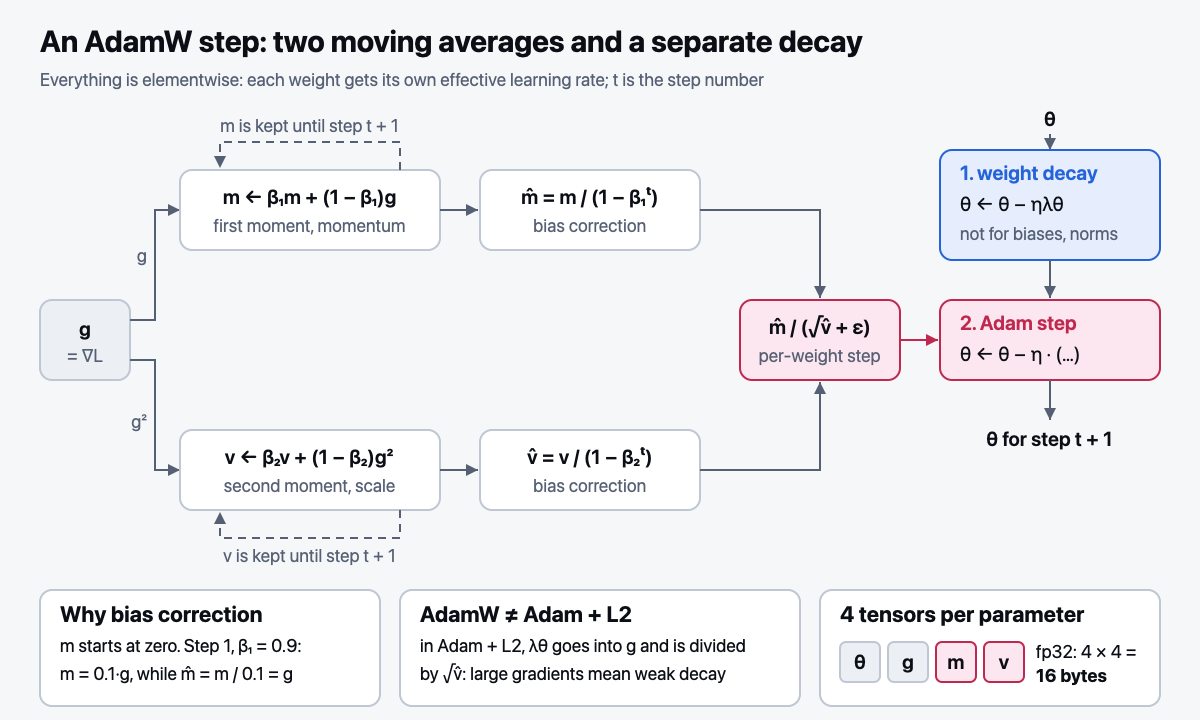
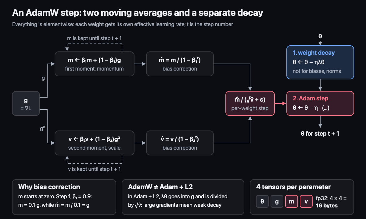
• Adam: the first moment m (momentum, a moving average of the gradients), the second moment v (a moving average of the squared gradients, scale normalization). In effect, every weight gets its own effective learning rate
• Bias correction: m̂ = m/(1−β₁ᵗ), needed because m, v are initialized with zeros
• Memory ≈ 4× the parameter size (θ, g, m, v). This is the basis of every training memory calculation

In plain terms. Weight decay (pulling the weights toward zero at every step) wants to shrink two weights by the same amount, λθ = 0.01. Adam with L2 puts λθ into the gradient and then divides everything by √v̂. For a weight with gradients around 10, the penalty becomes 0.01 / 10 = 0.001, and for a weight with gradients around 0.1 it becomes 0.01 / 0.1 = 0.1. A hundredfold difference: weights with large gradients are barely regularized. AdamW subtracts ηλθ separately, bypassing the division by √v̂, and equally for both.

• AdamW: weight decay as a separate term −ηλθ, applied before the Adam step
• Parameter groups (groups of parameters with their own settings): do not apply weight decay to biases or to norm parameters

• Heuristic: depends only on the step t → it is an LR schedule (learning rate schedule); needs per-parameter history → it is an optimizer
• Warmup (ramping the LR up from zero over the first steps; reduces the primacy effect of early examples), cosine decay (lowering the LR along a half cosine toward the end of training)

In plain terms. The gradient of two weights is (3, 4), its norm is 5, the clipping threshold is 1. Clipping by global norm divides the whole vector by 5: (0.6, 0.8). The length is now 1, the direction is unchanged. Elementwise clipping would cut each coordinate to 1: (1, 1). That is a different direction: the step will not go where the gradient pointed.

• Gradient clipping by global norm: if the norm of all gradients together exceeds the threshold, they are all multiplied by the same number threshold / norm

One sentence that ties Adam to week F4: Adam is diagonal preconditioning (a separate scale correction for each coordinate). Dividing by √v̂ equalizes the scale of the gradients across coordinates, which lowers the effective condition number of the problem (the ratio of the steepest curvature to the flattest). In the same picture, momentum looks like a "heavy ball" that does not react to every bump in the landscape. Further reading: Li, Mathematical Pathways to ML (2026), 12.5 and 11.5.

Code → nanolm/optim.py: write AdamW(torch.optim.Optimizer) from scratch: __init__ with defaults, step() with per-parameter state. Match torch.optim.AdamW to 1e-6. Exercise: exercises_en/optim.py, check: NANOLM_IMPL=exercises_en pytest tests/test_optim.py -v.

Math (track D): Markov, Chebyshev and Jensen inequalities. LLN and CLT.

Interview question of the week: "How does AdamW differ from Adam with L2 regularization, and why does it matter?" A 3-minute structure: (1) first say what Adam does: m, v, the step m̂/√v̂, every weight has its own effective learning rate; (2) L2 puts λθ into the gradient, and it also gets divided by √v̂: with gradients around 10 and 0.1 the penalty differs by a factor of 100, and weights with large gradients are barely regularized; (3) the conclusion: AdamW subtracts ηλθ separately, bypassing m and v, equally for all weights; (4) practice: parameter groups, no weight decay on biases and norms; a number: 4 tensors per parameter (θ, g, m, v), 16 bytes in mixed precision; (5) expect "so why bias correction". Without it v is underestimated more than m, and the first steps blow up to 3.2η, 4.2η, 5.0η instead of η.

Deeper: 05-ГЛУБИНА, section "Weeks 1–4, Track D. Math: a big shortfall".

Week outcomes

• I can implement AdamW as a torch.optim.Optimizer that matches the reference to 1e-6.
• I can compute what m equals at the first step without bias correction and explain why the correction is needed.
• I can compute the optimizer state memory for a model with N parameters in fp32.
• I can split parameters into groups with and without weight decay and justify the split.

Self-check

1. How does AdamW differ from Adam with L2 regularization, and why does the difference matter specifically for adaptive methods?
2. Why warmup, if Adam already normalizes its step?
3. What does clipping by global norm preserve that elementwise clipping does not?
4. Why is the mini-batch gradient an unbiased estimate of the full one, and how much larger must the batch be to halve the noise?
5. How many times does momentum with μ = 0.9 speed up descent down a steady slope, and what does it do to oscillations across a ravine?