Curriculum

Week 4. Information theory and numerical stability

Phase 1. Foundations · week 4 of 24

Learn in the app: tutor, coding problems →

Core: entropy, CE = KL + H, perplexity, logsumexp, online softmax · Depth: n-grams and smoothing, Gumbel-Softmax, the Boltzmann distribution · ≈ 11 h core / 22 h total

A language model's loss is cross-entropy, and without information theory you cannot understand what it means or why it equals ln V at the start (week 8). The second half of the week is about numerical stability: exp overflows in fp32 already at x ≈ 88.7, and a naive softmax produces NaN. Online softmax also comes from here, and it is the direct foundation of FlashAttention (week 13), while KL comes back in RLHF and DPO (week 17).

Theory

In plain terms. Three outcomes. The true distribution is p = (½, ½, 0), the model believes q = (¼, ¼, ½). The entropy H(p) is 1 bit: the best code for p spends 1 bit per outcome. A code built for q spends log₂ 4 = 2 bits on each of the first two outcomes. So the cross-entropy is CE(p, q) = ½·2 + ½·2 = 2 bits, and the overpayment is KL(p‖q) = 2 − 1 = 1 bit. The reverse KL(q‖p) is infinite: q puts ½ on the third outcome, to which p gives zero. KL is asymmetric. The loss uses the natural logarithm: to get the same quantities in nats, multiply by ln 2 ≈ 0.693.

• Entropy (the average surprise of an outcome, −Σ p log p), cross-entropy, KL (the Kullback–Leibler divergence: the average overpayment for encoding with q when the truth is p). The identity CE(p,q) = KL(p‖q) + H(p) must be derived
• CE loss with a one-hot target = negative log likelihood of the next token
• Probability of the whole sequence. By the chain rule (Module 0, F5) log p(x₁…x_T) = Σ_t log p(x_t | x_<t), where x_<t is all tokens before position t. CE averaged over positions equals exactly −(1/T) times this sum: by learning to predict the next token, the model maximizes the likelihood of the whole text

In plain terms. At every step the model honestly hesitates between four equally likely tokens: the correct one gets ¼. The mean loss is ln 4 ≈ 1.386, the perplexity is e^{1.386} = 4. Perplexity turns the loss into "the number of options the model chooses between on average". A loss of 3.4 gives e^{3.4} ≈ 30 options, and a uniform model over a vocabulary of V gives exactly V.

• Perplexity PPL = exp(−(1/T) Σ_t log p(x_t | x_<t)): the exponential of the mean CE per token. It is comparable only with the same tokenizer and the same test text: another vocabulary changes both T and the probabilities themselves (which is why different models are compared in bits per byte, week 5)

In plain terms. The corpus is a b a b a c. A bigram model (the next token depends only on the previous one) counts pairs: after a came b twice and c once, hence p(b|a) = 2/3, p(c|a) = 1/3, p(a|a) = 0. This is MLE (Module 0, F5): the count of the pair divided by the count of the first token. The test contains the pair a a: probability 0, infinite loss. Add-one (add 1 to the count of every possible pair, vocabulary of three tokens): p(a|a) = (0 + 1)/(3 + 3) = 1/6, p(b|a) = 3/6, p(c|a) = 2/6. The zero is gone, and the frequent pairs gave up some of their mass.

• N-gram model as a baseline: p(x_t | x_{t−n+1} … x_{t−1}) from counts, and training is just counting. Two problems: an unseen n-gram gets zero, and there are V^n possible n-grams, almost all of which occur zero times in the corpus
• Smoothing: add-α (count + α) / (count(prev) + α·V) (with α = 1 it is add-one, also called Laplace smoothing); backoff and interpolation (lean on a shorter context: λ·p(c|ab) + (1 − λ)·p(c|b)); Kneser–Ney (the best classical variant: the shorter context counts after how many different words a word has appeared). A neural LM removes both problems: softmax gives no zeros, and similar contexts get similar vectors
• The perplexity of a bigram model on your tokenizer is the bar nanolm must clear: if the trained transformer does not beat it, look for a bug in the code (the bigram_perplexity task in the trainer)
• Implementing the loss: shifting logits/labels, ignore_index (a label the loss skips, e.g. padding), a loss mask

In plain terms. exp(1000) does not fit in fp32 or even in fp64 (the limit there is about e^709), so you get inf. A naive softmax of [1000, 1001] gives inf / inf = NaN. Subtract the maximum: [1000, 1001] − 1001 = [−1, 0]. Now e^{−1} ≈ 0.368, e^0 = 1, and the answer is (0.269, 0.731). The answer is exactly the same: the numerator and the denominator were multiplied by the same number e^{−1001}, and it cancelled out.

• Numerical stability, where exactly it breaks:
  • exp(x) for large x → overflow (the result exceeds the type's maximum and becomes inf; in fp32 already at x ≈ 88.7, in fp16 at x ≈ 11)
  • log(x) as x→0 → underflow (a number too small becomes 0, and log 0 = −inf); as x→1 → loss of precision
• Stable softmax: subtract x_max (softmax is shift-invariant: you need to derive this)

In plain terms. Logits (0, 200). Even a stable softmax gives the first class a probability of e^{−200} ≈ 10⁻⁸⁷. fp32 has no such number (the smallest is about 10⁻⁴⁵): you get 0, and log 0 = −inf. Yet the answer exists and is simple: log_softmax = x − logsumexp(x), which for the first class is 0 − 200 = −200. Compute the logarithm directly, without going through the probability itself.

• log_softmax = x − logsumexp(x) (never materialize tiny probabilities)
• logsumexp(x) = x_max + log Σ exp(x − x_max)
• Softmax as the Boltzmann distribution. In physics, a state with energy E occurs with probability e^{−E}/Z, where Z = Σ e^{−E_j} (the partition function: the normalizing sum over all states). Softmax works the same way: a logit is minus the energy, Z = Σ e^{x_j}, and logsumexp(x) = log Z. Logits (3, 1, 0): Z ≈ 23.80, log Z ≈ 3.170, p ≈ (0.844, 0.114, 0.042). A shift by −3 gives (0, −2, −3): Z ≈ 1.185, log Z ≈ 0.170, exactly 3 less, while p stays the same. The sampling temperature (week 12) is the physical temperature from the same formula: the logits are divided by it

In plain terms. A stream of two numbers x = (1, 3) with values v = (10, 20); we need Σ softmax(x)ᵢ · vᵢ. After the first one: maximum m = 1, denominator d = e^{1−1} = 1, numerator o = 10. Then 3 arrives, a new maximum. The old d and o were computed relative to 1; we rescale them to 3 by multiplying by e^{1−3} ≈ 0.135: d = 0.135 + 1 = 1.135, o = 1.35 + 20 = 21.35. The answer is 21.35 / 1.135 ≈ 18.81. Directly: the weights are softmax(1, 3) = (0.119, 0.881), and 10·0.119 + 20·0.881 ≈ 18.81. They match, even though we never held the whole stream at once.

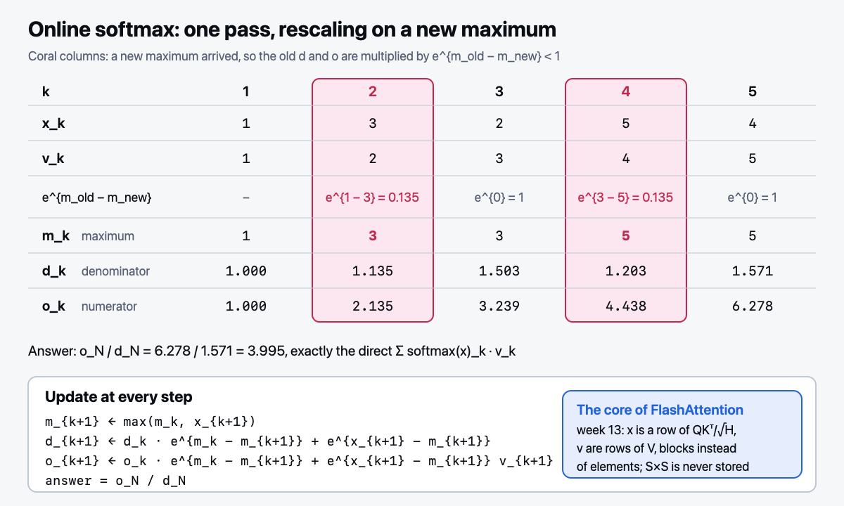
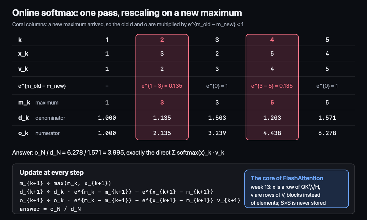
• The online softmax trick (softmax in one pass over a stream, without storing all the numbers) is the foundation of FlashAttention; study it thoroughly:

  m_{k+1} ← max(m_k, x_{k+1})
  d_{k+1} ← d_k · e^{m_k − m_{k+1}} + e^{x_{k+1} − m_{k+1}}
  o_{k+1} ← o_k · e^{m_k − m_{k+1}} + e^{x_{k+1} − m_{k+1}} v_{k+1}
  answer = o_N / d_N

  Derive the correctness of the d update in one line of algebra.

• The general recipe for stabilizing e^x: pick a shift m (almost always x_max), factor e^{m} out of the expression and check whether it cancels. In softmax it cancels completely; in logsumexp it remains as a separate term x_max. Both cases are the same transformation
• Gradients through sampling: Gumbel-Max (argmax of the logits plus Gumbel noise gives an exact sample from softmax), Gumbel-Softmax (it gives stochasticity, not differentiability: softmax is already differentiable), the straight-through estimator (a discrete choice in forward, the gradient of a smooth surrogate in backward)

Code → nanolm/stability.py: logsumexp, a stable softmax, log_softmax, online softmax for a streaming weighted average. Overflow tests (x = [1000, 1001]). Exercise: exercises_en/stability.py, check: NANOLM_IMPL=exercises_en pytest tests/test_stability.py -v.

Math (track D): MLE, bias-variance.

Interview question of the week: "How do you compute softmax without NaN, and what do you do if the vector does not fit in memory?" A 3-minute structure: (1) first name where it breaks: exp overflows in fp32 at x ≈ 88.7, in fp16 at x ≈ 11; a naive [1000, 1001] gives inf / inf = NaN; (2) the fix: subtract the maximum, e^{−m} cancels, the answer is (0.269, 0.731); (3) the second trap, underflow: with logits (0, 200) a probability of ≈ 10⁻⁸⁷ becomes zero, and log 0 = −inf; that is why the loss is computed via log_softmax = x − logsumexp(x), and the probability is never materialized; (4) a stream: online softmax keeps m, d, o, and on a new maximum multiplies the old ones by e^{m_old − m_new}; (5) the conclusion: this is the core of FlashAttention (week 13); expect to be asked to prove the d update at the whiteboard: it is one line: d_k·e^{m_k − m_{k+1}} = Σ_{i≤k} e^{x_i − m_{k+1}}.

Deeper: 05-ГЛУБИНА, section "Weeks 1–4, Track D. Math: a big shortfall".

Week outcomes

• I can derive CE(p,q) = KL(p‖q) + H(p) and explain why minimizing CE over q is the same as minimizing KL.
• I can derive the correctness of the online softmax denominator update in one line of algebra.
• I can implement logsumexp, softmax, log_softmax that pass the test on x = [1000, 1001].
• I can explain in 2 minutes why log(softmax(x)) must not be computed naively.

Self-check

1. At what x does exp overflow in fp32, and why does subtracting the maximum not change the answer?
2. What does online softmax store, and how are the accumulated quantities rescaled on a new maximum?
3. Why Gumbel-Softmax, if softmax is already differentiable?
4. The model gave the correct tokens probabilities ½, ¼, ⅛. What is the perplexity, and how do you explain it in words?
5. Why does a bigram model need smoothing, why does a transformer not need it, and what is wrong with add-one on a large vocabulary?

✅ Checkpoint 1

No hints, 90 minutes:

1. Derive ∂L/∂z for softmax+CE
2. Write AdamW from scratch
3. Explain why logsumexp is stable, and derive online softmax
4. Compute the training memory of a 1.5B-parameter model in bf16 (a 16-bit format with the exponent of fp32 and a short mantissa; details in week 14) with AdamW