Curriculum

Week 2. Backpropagation

Phase 1. Foundations · week 2 of 24

Learn in the app: tutor, coding problems →

Core: the computational graph, the softmax+CE gradient, your own autograd, activation checkpointing · Depth: forward-mode autodiff, continuous distributions (track D) · ≈ 11 h core / 21 h total

Backprop is the only way anything in this course learns, from MLPs to RLHF. Its bugs do not raise exceptions: a gradient that is overwritten instead of accumulated simply makes the model learn worse. This is also where p − one_hot(t) appears, which comes back in policy gradient (week 16), and checkpointing, without which the activations of large models do not fit in memory (week 9).

Theory

• The computational graph (a computation written as nodes that are operations, with numbers flowing along the edges). Splitting it into "gates" (nodes) is a matter of convenience: you put a gate where the local gradient is simple
• downstream = upstream × local. Here upstream is the gradient of the loss with respect to the node's output; local is the derivative of the node's output with respect to its input; downstream is the gradient of the loss with respect to that input

In plain terms. The graph: q = x + y, then f = q · z. Inputs x = 1, y = 2, z = 4; the forward pass gives q = 3, f = 12. Backward starts from the end, and the upstream at the output is 1. The × node: ∂f/∂z = q = 3, ∂f/∂q = z = 4: the factors swapped places. The + node: the local gradient for each input is 1, so ∂f/∂x = ∂f/∂y = 4 · 1 = 4. Check: x = 1.01 gives q = 3.01, f = 12.04. The change of 0.04 equals 4 · 0.01.

In plain terms. Let f = a · a with a = 3, so f = 9. The × node sees two inputs, and both are a. For the first input the local gradient is the second factor, 3; for the second it is the first factor, also 3. The correct gradient is the sum: 3 + 3 = 6, just like (a²)' = 2a = 6. If the second contribution overwrote the first, you would get 3. Off by a factor of two, and no exception.

• Gradients add up at branch points
• Node intuition: + distributes the gradient, max routes it to one input, × swaps the coefficients
• Reverse topological order. A topological order is one where every node comes after all of its inputs; the reverse one goes from the loss to the inputs, so that all contributions reach a node before it is processed

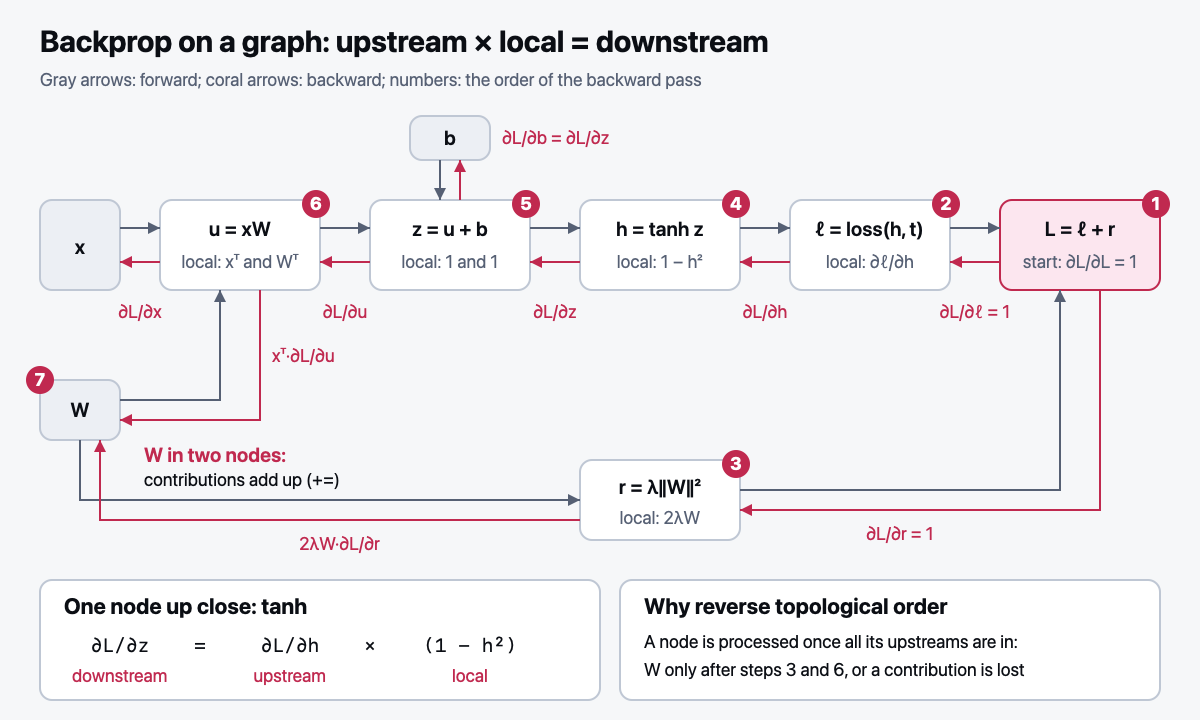
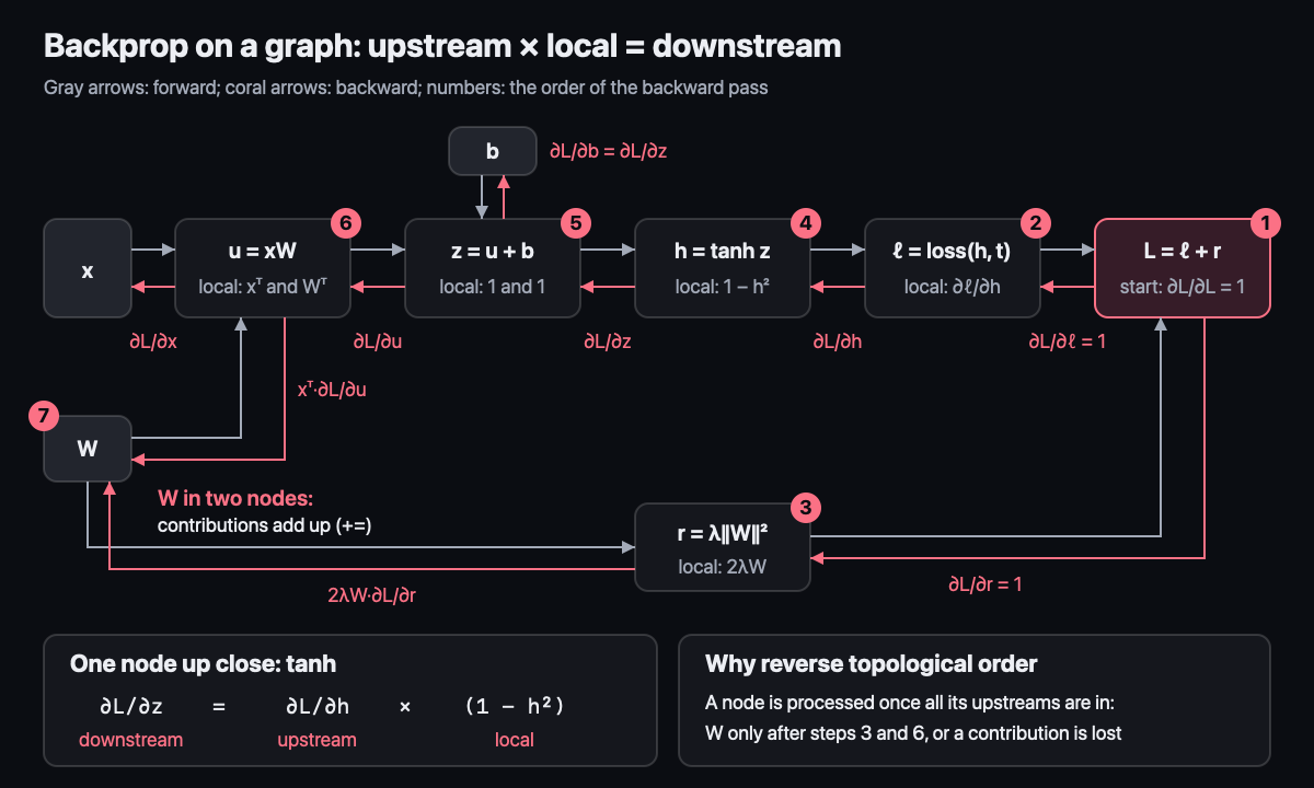
• Forward and backward have the same order of complexity
• Automatic differentiation: every node type knows its own local gradient
• Gradient checking (verifying the gradient numerically): f'(x) ≈ (f(x+h) − f(x−h)) / 2h

In plain terms. A network has a million weights. The numerical gradient nudges each weight in turn in both directions: that is 2·10⁶ forward passes per step. Backward returns all million derivatives in one pass, at the cost of roughly two forward passes: each node multiplies the upstream by its local gradient once. So the numerical gradient is only for checking on a tiny network, and training uses backprop.

• Forward and reverse mode automatic differentiation. Forward mode carries derivatives along with the forward pass, from input to output: one pass gives the derivatives of all outputs with respect to one input (a Jacobian-vector product, JVP). Reverse mode (the one called backprop) goes from the output to the inputs: one pass gives the derivatives of one output with respect to all inputs (a vector-Jacobian product, VJP). Training has one output (a scalar loss) and billions of inputs, so reverse mode is the choice. Its price: forward activations must be kept until backward

In plain terms. A network of 100 layers. A regular backward pass keeps all 100 activations in memory. Checkpointing saves every tenth one, 10 in total. In backward, each segment of 10 layers is recomputed from the nearest saved point, and its 10 activations temporarily sit in memory as well. The peak is 10 + 10 = 20 instead of 100, and the price is roughly one extra forward pass. With 5 checkpoints it would be 5 + 20 = 25, with 20 checkpoints 20 + 5 = 25: the minimum is exactly at √100 = 10.

• Activation checkpointing (store some activations and recompute the rest in backward): memory O(N) → O(K + N/K), optimal at K=√N → memory O(√N), backward compute about O(2N)
• Why .backward() requires a scalar: ∂L/∂θ is one number per parameter
• The gradient of the mean loss = the mean of the gradients (linearity of the derivative)

In plain terms. The model predicted ŷ = 2, the truth is y = 3. Suppose the truth equals the prediction plus Gaussian noise (a random addition with a bell-shaped distribution) of variance 1. The density of this outcome is e^{−(y−ŷ)²/2} / √(2π), and its negative log is (y − ŷ)²/2 + ½·ln 2π ≈ 0.5 + 0.919. The second term does not depend on the model, so minimizing the negative log-likelihood means minimizing the squared error. The derivative with respect to ŷ is ŷ − y = −1: prediction minus truth, exactly like p − one_hot(t) below.

• The loss function as NLL (negative log-likelihood: minus the log of the probability the model gave to the correct answer). Regression with Gaussian noise gives MSE, a categorical output gives cross-entropy, a Bernoulli output gives binary cross-entropy (Module 0, F6). The noise assumption picks the loss: Laplace noise (with heavy tails) would give |y − ŷ|, that is MAE, which is robust to outliers
• Why not train directly on accuracy (the share of correct answers): it is a step function. A small change of the weights does not change it, and the gradient is zero almost everywhere. The loss is chosen smooth and differentiable, the metric is computed separately

In plain terms. Three classes, logits z = (0.69, 0, 0). Since e^0.69 ≈ 2, softmax gives p = (2, 1, 1) / 4 = (0.5, 0.25, 0.25). The correct class is the second one, loss −ln 0.25 ≈ 1.386. The formula below promises the gradient p − one_hot(t) = (0.5, −0.75, 0.25). Let's check the second logit: raise it by 0.01, then p₂ becomes 0.2519 and the loss 1.3788. The loss dropped by 0.0075 = 0.75 · 0.01. The sign and the factor match. Descent pulls the correct logit up with strength 1 − p_t, and the others down with strength equal to their probability.

The key derivation of the week. Do it by hand: this gets asked all the time:

Gradient of softmax + cross-entropy:
  ∂L/∂z = p − one_hot(t)

Path: ∂L/∂p (nonzero only at t) → the softmax Jacobian (p_j(1−p_j) on the diagonal, −p_j p_i off it) → everything collapses.

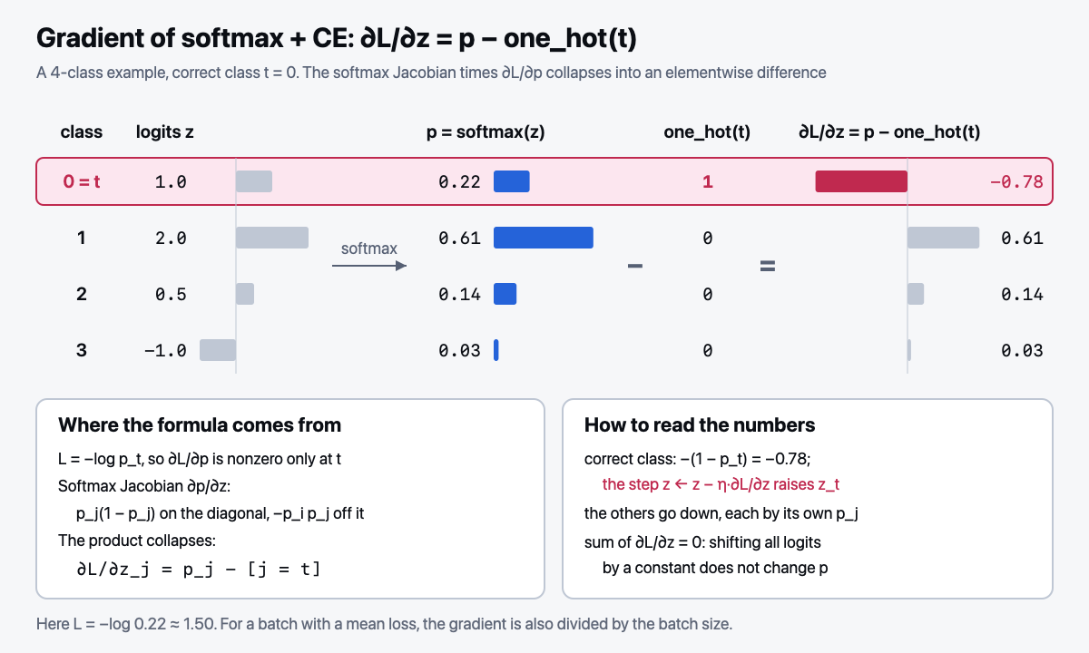
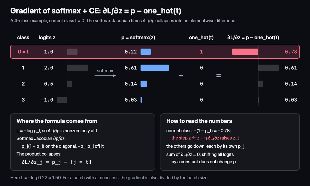
Code → nanolm/autograd.py: your own autograd engine (micrograd style): a Value holding a scalar, a gradient and references to its parents; operations + * tanh exp pow, each of which knows its own local gradient; .backward() builds a topological sort of the graph and walks it in reverse. Then Neuron, Layer, MLP on top of Value and training on XOR. Exercise: exercises_en/autograd.py, check: NANOLM_IMPL=exercises_en pytest tests/test_autograd.py -v.

What to look for in the tests: a node used twice (a * a, a + a) must receive the sum of its gradients: this is the branching rule from the theory above. If the gradient is overwritten instead of +=, test_reused_variable_accumulates_gradient fails. The diamond-shaped graph (test_diamond_graph_needs_topological_order) catches a traversal without a topological sort, and random expressions are compared against PyTorch.

Math (track D): Uniform, Exponential, Gaussian. The memoryless property (geometric and exponential are the only memoryless distributions).

Interview question of the week: "Derive the gradient of softmax + cross-entropy with respect to the logits." It is asked word for word. A 3-minute structure: (1) the answer first: ∂L/∂z = p − one_hot(t); (2) the path: ∂L/∂p is nonzero only at t and equals −1/p_t → row t of the softmax Jacobian (p_t(1−p_t) on the diagonal, −p_t p_j off it) → after multiplying, what remains is p_j − [j = t]; (3) the meaning: the correct logit is pulled up with strength 1 − p_t, the others down with strength p_j, and the gradient sums to zero; (4) a number: z = (0.69, 0, 0), correct class is the second → (0.5, −0.75, 0.25); raise the second logit by 0.01 and the loss drops by 0.0075; (5) expect "why is this one function of the logits in code rather than softmax followed by log". Answer: log_softmax via logsumexp (week 4), with no division by a tiny p_t.

Deeper: 05-ГЛУБИНА, section "Weeks 1–4, Track D. Math: a big shortfall".

Week outcomes

• I can derive ∂L/∂z = p − one_hot(t) for softmax + CE through the softmax Jacobian in 5 minutes.
• I can implement Value autograd with a topological sort and train an MLP on it.
• I can show on a graph why gradients add up at a branch point, and find this bug in someone else's code.
• I can compute the memory and compute cost of activation checkpointing and derive the optimum K = √N.

Self-check

1. Why does backward go in reverse topological order, and what breaks with a different order?
2. How do the +, × and max nodes distribute the gradient in the backward pass?
3. Why does gradient checking use a central difference, and why in float64?
4. Why is MSE the negative log-likelihood of a Gaussian, and why can a model not be trained directly on accuracy?
5. How many forward passes does a numerical gradient for N weights cost, and why does training need reverse mode rather than forward mode?