Curriculum

Week 1. Neural networks and gradients

Phase 1. Foundations · week 1 of 24

Learn in the app: tutor, coding problems →

Core: an MLP and tensor shapes, Jacobians and the chain rule, activation functions, an MLP in numpy with backward · Depth: distributions and expectation (track D) · ≈ 10 h core / 20 h total

Everything the model does later boils down to matrix multiplications, nonlinearities and their gradients. If shapes and Jacobians do not become automatic here, every following week (backprop, attention, LoRA) turns into guessing where to transpose. This week builds one skill: derive the gradient of a layer on a batch and check it by shape.

Theory

• MLP (multilayer perceptron: "linear transform → nonlinearity" layers stacked in a row): neuron = f(wᵀx + b), layer = H = f(XW + b)
• The batch dimension: why PyTorch stores W as (n_out, n_in) and transposes it. Transposing is free: only the stride changes (the step in memory between neighboring elements along an axis), no data is copied. And the gradient ∂L/∂W comes out in the right shape directly
• Activation functions: sigmoid, tanh, softmax (+ temperature), ReLU, LeakyReLU, Swish (x·σ(x)), GLU (the output of one projection multiplied by a gate from another), SwiGLU

In plain terms. A layer "multiply by 2", followed by a layer "multiply by 3": together they are one layer "multiply by 6". No matter how many linear layers you stack, the total is a single matrix. A nonlinearity breaks this. ReLU(x) − ReLU(x − 1) equals 0 at x = −1, 0.5 at x = 0.5 and 1 at x = 2. That is a step, and no straight line can draw a step.

• Why depth is useless without nonlinearities: W₁W₂x = Wx

In plain terms. The derivative of the sigmoid is never larger than 0.25. In the backward pass, each sigmoid layer multiplies the gradient by σ', so at best by 0.25. After 10 such layers what remains is 0.25¹⁰ ≈ 10⁻⁶ of the original signal. The first layers barely learn.

• Problems: vanishing gradients with sigmoid (σ' ≤ 0.25), non-zero-centered output (the sigmoid output is always positive, so the gradients of all input weights of a neuron have the same sign), dying ReLU (the neuron has drifted into a region where it outputs 0 on every input, and no gradient reaches it anymore)

In plain terms. A function from two numbers to two: f(x, y) = (x·y, x + y²). At the point (2, 3) it outputs (6, 11). Shift x by 0.01: the output becomes (6.03, 11.01), a change of (0.03, 0.01). Shift y by 0.01: the output is (6.02, 11.0601), a change of (0.02, 0.0601). Divide the changes by the step: the column for x is (3, 1), the column for y is (2, 6.01). The extra 0.01 comes from the square: it is the 0.01² contribution; with a smaller step it vanishes. The result is the table [[3, 2], [1, 6]]. That is the Jacobian: each row corresponds to one output, each column to one input. As a formula: J = [[y, x], [1, 2y]].

• Gradient (the vector of derivatives of a scalar function with respect to all inputs), Jacobian (m×n: the derivative of each of the m outputs with respect to each of the n inputs), Hessian (n×n, second derivatives, i.e. the curvature of the loss landscape)
• The chain rule: for multivariate functions it is a product of Jacobians
• The Jacobian of an elementwise function = diag(f'(z)): output i depends only on input i, so everything off the diagonal is zero

Derive on paper (required)

• ∂/∂x (Wx+b) = W, ∂/∂b (Wx+b) = I, ∂/∂u (uᵀh) = hᵀ
• The derivative of the sigmoid via the quotient rule: σ' = σ(1−σ)
• The derivative of Swish via the product rule: σ(x) + Swish(x)(1−σ(x))

In plain terms. One weight w = 3, a batch of two numbers x = (1, 2), outputs zᵢ = w·xᵢ, loss L = z₁ + z₂ = 9. Shift w by 0.01: both outputs move, and L grows by 0.01·(1 + 2). So ∂L/∂w = 1 + 2 = 3: the contributions of the examples add up to a single number, because w itself is shared by the whole batch. Shift only x₁: only z₁ changes, so ∂L/∂x₁ = 3. Likewise ∂L/∂x₂ = 3. The result is (3, 3): one number per example, the same shape as x.

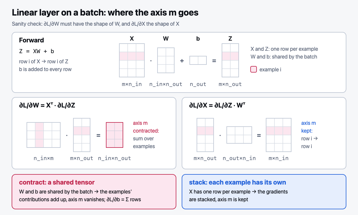
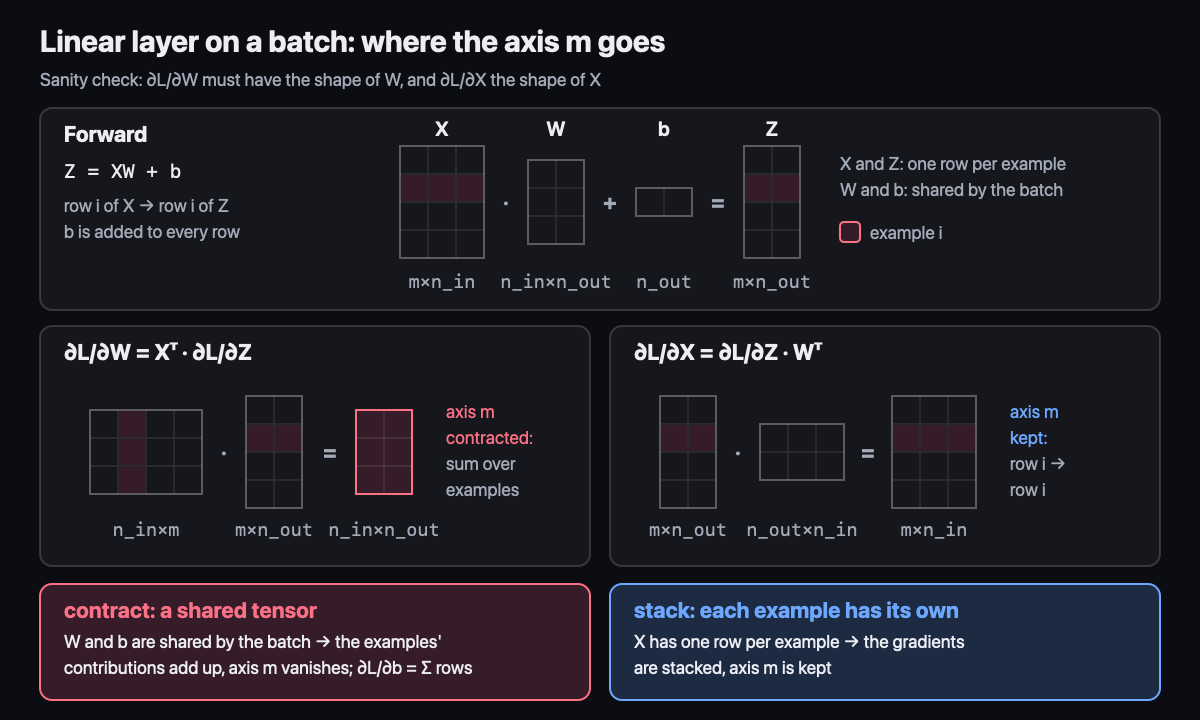
How not to get lost in shapes with a batch. Derive the Jacobian for a single example: everything there is two-dimensional and obvious. After that the only question is where the batch axis goes, and the answer follows directly from how many times the tensor takes part in the computation:

• W is shared by the whole batch, and each example contributes its own share to ∂L/∂W → the contributions add up, the batch axis disappears (it is contracted inside the matmul).
• Each example has its own row of X, and rows of Z do not mix across examples → the gradients are simply stacked, and the batch axis is kept.

Sanity check: ∂L/∂W must have the shape of W, and ∂L/∂X must have the shape of X. If you got something else, an axis was lost or one is extra.

Code (track B): an MLP in plain numpy: forward and backward by hand, no autograd. Check it with a numerical gradient (the difference (f(w+h) − f(w−h)) / 2h for every weight).

Math (track D): Bernoulli, Binomial, Poisson, Geometric. Derive E[X] and Var[X] for each. Trick: X² = X for indicators. Trick: decompose into Bernoullis and use linearity.

LeetCode: arrays, hash tables, two pointers (3 problems from the Track C list).

Interview question of the week: "Derive the gradients of the linear layer Z = XW + b on a batch. What shapes do ∂L/∂W and ∂L/∂X have?" A 3-minute structure: (1) name the shapes first: X is (m, n), W is (n, k), Z is (m, k); (2) derive on a single example, where everything is two-dimensional, then ask one question: where does the batch axis go; (3) the key conclusion: W is shared by the batch → contributions add up, ∂L/∂W = Xᵀ·∂L/∂Z; each example has its own X → a stack, ∂L/∂X = ∂L/∂Z·Wᵀ; ∂L/∂b is the sum over the batch; (4) the check: a gradient must have the shape of its tensor, plus a numerical gradient via central differences, relative error < 1e-6 in float64; (5) expect the follow-up "why does PyTorch store W as (n_out, n_in)". Answer: transposing is free, only the stride changes.

Deeper: 05-ГЛУБИНА, section "Weeks 1–4, Track D. Math: a big shortfall".

Week outcomes

• I can derive on paper ∂(Wx+b)/∂x, ∂/∂W, ∂/∂b, and the derivatives of sigmoid and Swish in 10 minutes with no hints.
• I can tell from the shapes where the batch axis is summed (∂L/∂W) and where it is kept (∂L/∂X), and check the result by shape.
• I can implement an MLP in numpy with a hand-written backward and confirm it with a numerical gradient (relative error < 1e-6 in float64).
• I can explain in 2 minutes why depth is useless without a nonlinearity and why the sigmoid leads to vanishing gradients.

Self-check

1. Why, for a batch, is ∂L/∂W a sum of the examples' contributions, while ∂L/∂X is a stack? Name the shapes of both.
2. What is the Jacobian of an elementwise function, and why is it diagonal?
3. Three problems of the sigmoid in a hidden layer: which of them does ReLU solve, and what problem does ReLU introduce?