Curriculum

Week 7. Attention

Phase 2. The modern transformer · week 7 of 24

Learn in the app: tutor, coding problems →

Core: dividing by √H and the mask, MHA/MQA/GQA, RoPE, trade-offs of positional encodings · Depth: QK-norm, graph networks and the transformer as a GAT · ≈ 12 h core / 23 h total

Attention is the only place where tokens exchange information; everything else in the block works on each token separately. This is where the main inference costs come from (the KV cache, week 11), the main GPU bottleneck (week 13) and all the problems of long context (week 20).

Step 1. Scaling and the mask

In plain terms. Add up 64 random numbers, each +1 or −1: the sum is usually around ±8, not ±1. The dot product q·k is the same kind of sum of H terms, and its spread grows like √H. Softmax over numbers around ±8 produces something close to one-hot: one key takes all the attention, the rest get zero. Almost no gradient gets through such a softmax. Dividing by √H brings the numbers back to around ±1.

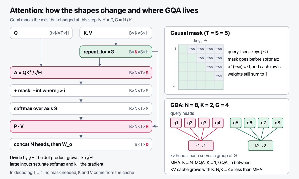
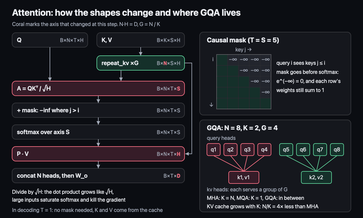
• Scaled dot-product: A = QKᵀ/√H. Why we divide: dot products grow like √H, large inputs to softmax → a peaked distribution → near-zero gradients. Derivation (D5): with independent coordinates of unit variance, Var(q·k) = Σ Var(qᵢkᵢ) = H
• The causal mask: −inf before softmax. Then e^{−inf} = 0, and each row is normalized over the past only. A mask after softmax would zero the weights, but the row would no longer sum to one

Step 2. How many K/V heads

In plain terms. 32 readers (query heads) search through card catalogs (key/value heads). In MHA each one has their own catalog, 32 in total, and all of them have to be kept in the cache. MQA: one catalog for everyone, a cache 32 times smaller, but everyone searches the same cards, and quality drops. GQA: 8 catalogs, one per group of 4 readers, a cache 4 times smaller, and the diversity is almost preserved.

• MHA → MQA → GQA: K, V are expanded from K heads to N heads. The motivation: the size of the KV cache. The cache and the W_k, W_v matrices shrink by exactly N/K (for Llama-3-8B, 32/8 = 4). A GQA model can be obtained from an MHA checkpoint by averaging the heads within each group and fine-tuning a little

Step 3. Position as a rotation

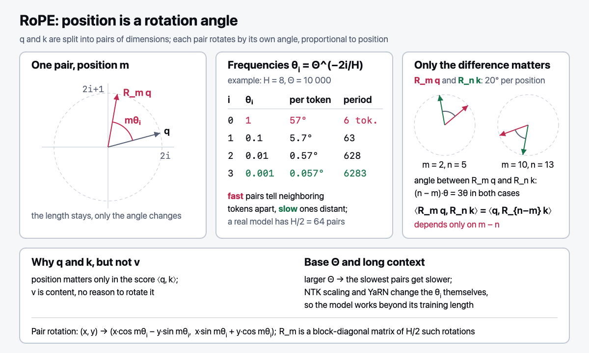
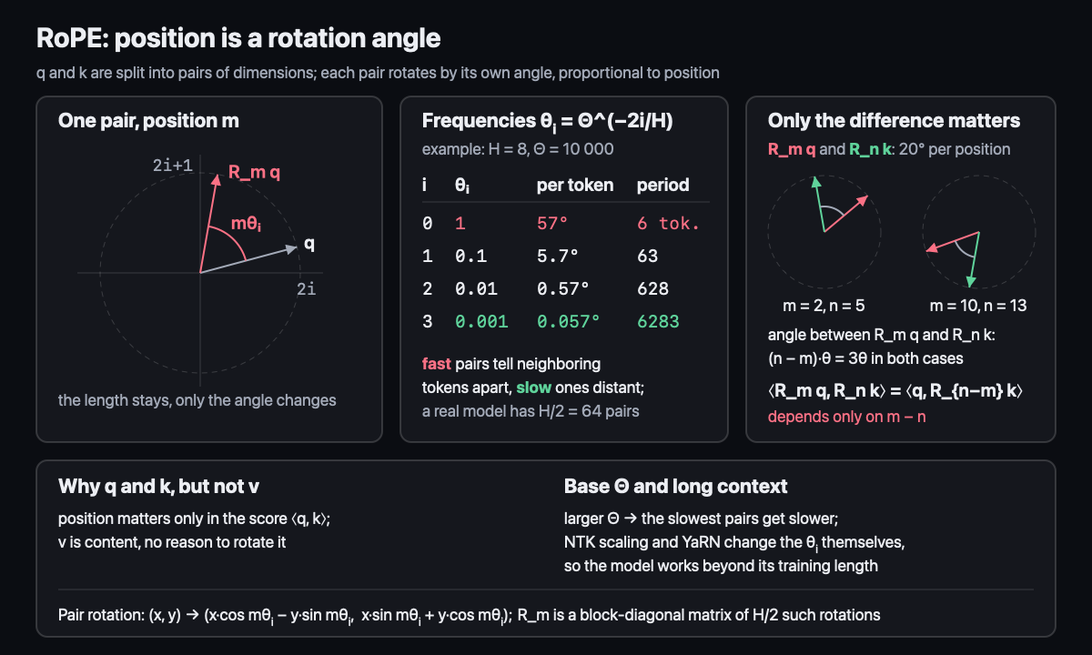
In plain terms. Each pair of coordinates holds a clock hand. The token's position sets how many times to rotate it: a token at position 3 is rotated by 3 steps, one at position 7 by 7 steps. The dot product sees only the angle between the hands, that is, the difference 7 − 3 = 4. Positions 103 and 107 give the same angle. The pairs rotate at different speeds: fast ones, like a second hand, tell neighbors apart; slow ones, like an hour hand, tell long distances apart.

• RoPE: rotating pairs of dimensions by the angle mθᵢ, where θᵢ = Θ^(−2i/H)
  • Derive why ⟨R_m q, R_n k⟩ depends only on m−n: this is exactly the relativity of positions. The key step: (R_m q)ᵀ R_n k = qᵀ R_mᵀ R_n k = qᵀ R_{n−m} k, because a rotation is orthogonal (R_mᵀ = R_{−m}), and rotations in the same plane add their angles. In complex form a pair becomes a number q̃ᵢ, the rotation becomes multiplication by e^{imθᵢ}, and the score equals Re Σ q̃ᵢ · conj(k̃ᵢ) · e^{i(m−n)θᵢ}
  • The role of the base Θ, context extrapolation, NTK scaling, YaRN. The slowest pair completes a full turn in roughly 2πΘ positions; increasing Θ stretches all the periods (details in week 20)
  • Compare with absolute / learned / ALiBi positional encoding

• Only q and k are rotated, not v: position decides who interacts with whom, not what gets passed along
• QK-norm: RMSNorm on q and k before the dot product, to keep scales under control. Without it, the attention logits of large models can grow without bound, and training falls apart
• Sliding window, attention sinks. A window caps the cache at the window size. A sink: softmax has to put its mass somewhere, and models dump it on the first tokens, so those cannot be dropped from the window

Extension (optional). Attention as message passing on a graph

nanolm does not need this step, but it changes how you see attention: a transformer turns out to be a graph network (GNN, graph neural network) on a complete graph. In this section A is the adjacency matrix (the table of "who is connected to whom"), not the attention scores from step 1.

In plain terms. Four nodes in a ring: 0–1–2–3–0. The adjacency matrix A of size S × S (here S = 4) holds 1 wherever there is an edge: in the row of node 0 the ones sit in columns 1 and 3. Each node has one feature, X = [1, 2, 3, 4]. A message-passing step: every node gathers the features of its neighbours and its own and averages them. Node 0 gets (1 + 2 + 4)/3 = 7/3, node 1 gets (2 + 1 + 3)/3 = 2. In one layer a node learns only about its neighbours; in k layers, about nodes up to k edges away.

• GCN (graph convolutional network; Kipf, Welling, 2017): X′ = Ã X W, where  = A + I, d_i is the sum of row i of Â (the node's degree including the self-loop), Ã[i, j] = Â[i, j] / √(d_i · d_j). Papers write this as D^(−1/2) (A + I) D^(−1/2) with a diagonal degree matrix; in this course D is the model width, so here the degrees are a vector d. The self-loop (an edge from a node to itself) keeps the node's own feature. The symmetric normalization stops nodes with a hundred neighbours from inflating the sum. In the ring all degrees are 3, and Ã gives exactly the mean from the example; in the path 0–1–2 the degrees are 2, 3, 2, and edge 0–1 weighs 1/√6 ≈ 0.41. W of shape (D, D′) is shared by all nodes, like one projection shared by all tokens
• Isotropic aggregation (a neighbour's weight is set by degrees only, not by content): GCN cannot decide that one neighbour matters more than another. Two neighbours with the same degree always get the same weight
• GAT (graph attention network; Veličković et al., 2018): attention computes the neighbour weights. Only the pairs "node and its neighbour" and a node with itself get a score, softmax runs over the neighbours, and every other pair gets −inf. This is anisotropic aggregation: two neighbours with the same degree can get weights 0.9 and 0.1. In the GAT paper a small network over concatenated features scores a pair, not q·k/√H, but the point is the same: the weight depends on node content
• A transformer is GAT on a complete graph. If every token is connected to every other, the mask is empty, and attention over neighbours becomes ordinary softmax(QKᵀ/√H) V. The causal mask defines the graph "a token sees itself and the earlier ones" (the lower triangle); a sliding window defines a band graph as wide as the window. A graph stores only connections, it has no order: that is why a transformer needs RoPE, and graph networks sometimes add positional features to nodes
• Cost and benefit. A complete graph has S² pairs, a sparse graph with E edges only E. In exchange, in a transformer any two tokens are connected within one layer. In a GCN the signal crosses one edge per layer, and with many layers node features get averaged until they are nearly identical (oversmoothing)

Trainer: the tasks gcn_layer and graph_attention; the second checks that a complete graph gives ordinary attention and the graph "I see earlier tokens" gives causal attention. Slides on the topic: Xavier Bresson's lecture on graph convolutional networks (link in Resources).

Common mistakes

• Forgetting /√H: caught by test_attention_scale_is_one_over_sqrt_head_dim, test_naive_attention_matches_pytorch
• repeat_kv by interleaving heads (x.repeat) instead of repeating each head consecutively: the groups get mixed up, caught by test_repeat_kv_groups_correctly
• Rotating the wrong pairs or getting a sign wrong: test_rope_preserves_norm, test_rope_is_identity_at_position_zero, and the main one, test_rope_makes_attention_relative
• view(B, N, T, H) directly instead of view(B, T, N, H).transpose(1, 2): mixes tokens across heads; leaking the future is caught by test_attention_is_causal

Code → nanolm/modules.py: attention with GQA and RoPE from scratch. RoPE (cos/sin tables, forward(x, offset)), repeat_kv, Attention (w_q, w_k, w_v, w_o, a qk_norm option), naive_attention. Exercise: exercises_en/modules.py, check: NANOLM_IMPL=exercises_en pytest tests/test_modules.py -v. Test: the result matches F.scaled_dot_product_attention to 1e-5.

Math (track D): D5: the variance of the dot product and the derivative of softmax with and without scaling; D6: the relativity of RoPE, the complex form and the longest "wavelength".

Interview question of the week: "Name all the ways to encode position and their trade-offs." You need to talk for 4 minutes without pauses. Structure: where position enters (the input or the attention scores) → sinusoidal and learned (absolute; learned is limited to the training length) → relative biases (T5, ALiBi: a penalty linear in distance) → RoPE (rotation, relativity through orthogonality, compatible with the KV cache) → NoPE (the causal mask itself provides a positional signal) → extrapolation for each.

Sources: Vaswani et al. (2017); Shazeer, MQA (2019); Ainslie et al., GQA (2023); Su et al., RoFormer (2021); Press et al., ALiBi (2021); Xiao et al., Attention Sinks (2023); Kipf, Welling, GCN (2017); Veličković et al., GAT (2018).

Deeper: 05-ГЛУБИНА, sections "Week 7. RoPE: the frequency design" and "Small additions".

Week outcomes

• I can derive that ⟨R_m q, R_n k⟩ depends only on m − n, in complex form, in 5 minutes.
• I can implement attention with GQA and RoPE that matches F.scaled_dot_product_attention to 1e-5.
• I can compute by how much GQA shrinks the KV cache for given N and K.
• I can talk for 4 minutes without pauses about the ways to encode position and their trade-offs.

Self-check

1. Derive from the variance of the dot product why the scores are divided by √H.
2. Why does RoPE rotate q and k but not v?
3. How does GQA reduce to MHA and to MQA at the extreme values of K?
4. (Extension) How does a GCN layer differ from a GAT layer? Why can a transformer be called GAT on a complete graph, and which graph does the causal mask define?
5. (Extension) Why does GCN add self-loops and divide an edge weight by √(d_i · d_j)? Compute the weights in the row of node 1 for the path 0–1–2.