Curriculum

Week 6. Architecture, part I

Phase 2. The modern transformer · week 6 of 24

Learn in the app: tutor, coding problems →

Core: the residual stream and pre-norm, RMSNorm, SwiGLU and F = 8D/3, the B/L/T/S/V/D/H/F/N/K/G notation · Depth: weight tying, the geometry of RMSNorm (D3) · ≈ 10 h core / 19 h total

Every element of the modern block (pre-norm, RMSNorm, SwiGLU) answers a specific problem of the 2017 transformer; none of it is fashion. Without understanding why they are there, you will not be able to debug the training of a deep model (week 10) or count its parameters (week 9).

Notation (learn it by heart, every discussion uses it):

Step 1. The residual stream and where normalization goes

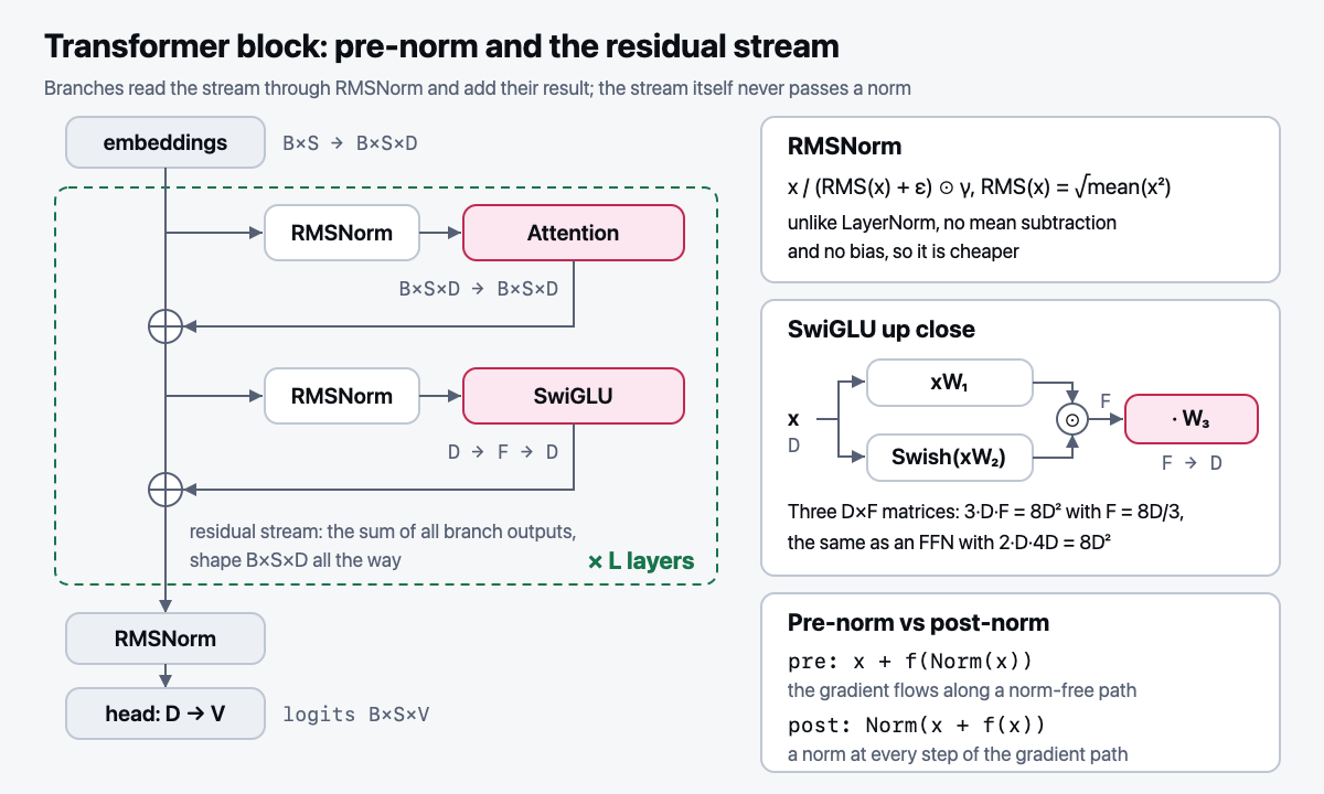
In plain terms. The residual stream is a shared notebook that L authors receive one after another. None of them rewrites the page; each one adds a correction. In post-norm, after every author the whole notebook is reprinted through a filter, and the error signal travels back to the first author through all L filters. Each filter multiplies it by its own factor, and the factors compound: at 0.9 per layer, after 32 layers you are left with 0.9³² ≈ 0.03. In pre-norm the filter sits only at the author's input: the author reads a normalized copy but adds the correction to the original.

• Embeddings, the residual stream as the model's "bus": x_{l+1} = x_l + f_l(x_l). The layer's Jacobian is I + ∂f/∂x, so the gradient always has a path through the identity (the same idea as in LSTM, week 19)
• Pre-norm vs post-norm, and why everyone switched to pre-norm. Post-norm LN(x + f(x)) puts the norm right on the gradient path: at initialization the gradients of the last layers are large, and you need a long warmup (ramping the learning rate up from zero). Pre-norm x + f(LN(x)) keeps the path clean. The price: the norm of the stream grows with depth, later layers change it less and less, and a final norm is needed before the head

In plain terms. The vector [3, 4]: its root mean square is √((9 + 16)/2) ≈ 3.54. RMSNorm divides by it and gets [0.85, 1.13]: standard scale, same direction. LayerNorm would first subtract the mean 3.5 and get [−1, 1]: the fact that both numbers were positive is lost. Experience has shown that centering gives almost nothing but costs a separate pass over the vector.

• RMSNorm: x / √(mean(x²) + ε) ⊙ γ. How it differs from LayerNorm (no mean subtraction and no bias) and why it is cheaper: one reduction (collapsing a vector into a number) instead of two. Geometrically (D3): the output of RMSNorm lies on a sphere of radius √D, and LayerNorm's output on the same sphere inside the hyperplane ⊥ 𝟏. The learnable γ gives the model back per-dimension scale, all the way down to zeroing a dimension out

Step 2. The gated FFN

In plain terms. Swish (Swish(x) = x·σ(x), where σ is the sigmoid) is a smooth version of ReLU: a large positive number passes almost entirely, a negative one is damped almost to zero. Let F = 2, and for one token let the value be xW₁ = (3, 3) and the gate xW₂ = (2, −2). Swish of the gate: 2·σ(2) ≈ 2·0.88 = 1.76 and −2·σ(−2) ≈ −2·0.12 = −0.24. The elementwise product is (3·1.76, 3·(−0.24)) ≈ (5.28, −0.72): the same value 3 passed through amplified in the first coordinate and was almost shut off in the second. Then W₃ maps the vector back to size D. The value answers "what to pass on", the gate answers "how much".

• SwiGLU FFN: (xW₁) ⊙ Swish(xW₂), then W₃. Three matrices instead of two → F = ⅔ · 4D = 8D/3 to keep the parameter count. Derivation: 2·D·4D = 8D² = 3·D·F. It is rounded up to a multiple of 256: with D = 4096 you get 11008. One projection carries the value, the other decides through Swish how much of it to let through. This is a multiplicative interaction, and at an equal parameter count it beats the ReLU FFN in quality

• Weight tying of the input and output embeddings (one matrix for the input and for the head): saves V·D, which in GPT-2 small is about a third of all parameters. In large models the share is small, and the matrices play different roles: one reads the token, the other predicts the next one. That is why tying is often dropped there

Common mistakes

• Subtracting the mean "out of habit": you get LayerNorm without a bias, caught by test_rmsnorm_does_not_center. Normalizing along the wrong axis: test_rmsnorm_produces_unit_rms; forgetting γ: test_rmsnorm_scales_with_gamma
• Computing the norm in bf16 (16 bits: the exponent of fp32, a short mantissa; details in week 14): the sum of squares loses precision. The reference casts the input to fp32 and back
• Adding the normalized x to the stream instead of the raw one: the path through the identity disappears. There is no dedicated test: it is caught by comparing logits in week 8
• Taking F = 4D with three matrices: 1.5 times as many parameters, caught by test_swiglu_ffn_dim_is_8D_over_3 (in test_budget.py)

Code → nanolm/modules.py: RMSNorm and SwiGLU from scratch (w_gate, w_up, w_down), checked against the reference implementation. The configuration lives in ModelConfig in config.py (H, G, ffn_dim, tie_embeddings), the assembly in Block in model.py. Exercise exercises_en/modules.py, check: NANOLM_IMPL=exercises_en pytest tests/test_modules.py -k "rmsnorm or swiglu" -v.

Math (track D): D3: the geometry of LayerNorm and RMSNorm via a projector; D4: Markov, Chebyshev and norm concentration: why ‖x‖² ≈ D at initialization.

Interview question of the week: "Why did everyone switch to pre-norm, and what does it break?" A 3-minute structure: post-norm in the original → a norm on the gradient path, warmup needed → pre-norm: a path through the identity → the price: the stream's norm grows, a final norm → variants that also put a norm at the branch output (Gemma 2, OLMo 2).

Sources: Xiong et al., On Layer Normalization in the Transformer Architecture (2020); Zhang & Sennrich, RMSNorm (2019); Shazeer, GLU Variants Improve Transformer (2020).

Deeper: 05-ГЛУБИНА, section "Small additions", row "Week 6".

Week outcomes

• I can implement RMSNorm and SwiGLU that match the reference.
• I can derive F = 8D/3 from the condition that SwiGLU and a regular FFN have equal parameter counts.
• I can explain pre-norm versus post-norm in 2 minutes through the gradient path along the residual stream.
• I can name the full notation B, L, T, S, V, D, H, F, N, K, G without hints.

Self-check

1. What does RMSNorm remove compared with LayerNorm, and why does it have a learnable γ?
2. Why does pre-norm train more stably than post-norm?
3. What does weight tying give you, and why do large models often drop it?