Curriculum

Week 16. RL: from REINFORCE to PPO

Phase 4. Post-training · week 16 of 24

Learn in the app: tutor, coding problems →

Core: the policy gradient with its derivation, an unbiased baseline, importance sampling, PPO and clipping · Depth: GAE in detail, generative models beyond autoregression (05-ГЛУБИНА) · ≈ 12 h core / 23 h total

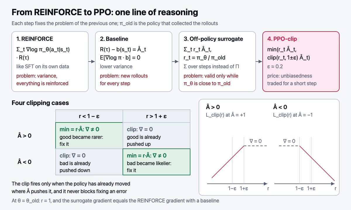
Here the order matters more than the content. The usual story is REINFORCE, then straight to PPO, and clipping looks like an arbitrary trick you memorize. There is an intermediate step between them, and with it the whole progression becomes one line of reasoning.

Step 1. Policy gradient

In plain terms. A bandit with three arms A, B, C: a single action, no states. The policy is softmax(θ); at the start θ = (0, 0, 0) and π = (⅓, ⅓, ⅓). Arm A comes up, reward R = 1. The gradient is ∇θ log π(A) = one_hot(A) − π = (⅔, −⅓, −⅓), exactly what cross-entropy with label A would give. REINFORCE takes the step θ ← θ + η·R·(⅔, −⅓, −⅓). With η = 1 you get θ = (0.67, −0.33, −0.33), and π(A) rises from 0.33 to 0.58. This is SFT on the model's own sample, multiplied by the reward. With a reward of 0 there is no step; with a negative one the step moves away from A.

• MDP (Markov decision process: state, action, reward, transition), policy (a distribution over actions in a given state), value (the expected future reward from a state), advantage (how much better an action is than average in that state). An LLM as a policy over tokens: the action is the next token, the state is the prefix written so far
• Derive the theorem by hand via the log-derivative trick: ∇P = P∇log P
• REINFORCE. Notice that this is the same update as in SFT, except that the data is sampled by the policy itself and the gradient is weighted by the reward

The discount γ (a factor between 0 and 1: how much a reward loses in value for each step of waiting). In plain terms. γ = 0.9. A reward of 1 now is worth 1, one step later 0.9, 3 steps later 0.9³ ≈ 0.73, 10 steps later 0.9¹⁰ ≈ 0.35. Just as in economics: a dollar a year from now is worth less than a dollar today. Now take an LLM response of 500 tokens with a single reward at the very end. With γ = 0.99, only 0.99⁵⁰⁰ ≈ 0.007 of it reaches the first token: the signal has almost vanished. Formula: the return (the sum of future rewards) G_t = r_t + γ·r_{t+1} + γ²·r_{t+2} + … = Σ_k γ^k·r_{t+k}, value V(s) = E[G_t | s_t = s]. In classical RL γ < 1 is needed so the infinite sum converges and a near reward is valued above a distant one. For an LLM the episode is finite and there is one reward, so RLHF and RLVR usually use γ = 1: every token of the response gets the same final score. λ in GAE (step 2) is a different factor: it is not about the value of the future but about mixing horizons in the advantage estimate.

The Bellman equation and value iteration. The value from the formula above obeys a simple rule: the value of a state equals the reward for the next step plus the discounted value of wherever that step leads. In plain terms. Two states, s₁ and s₂, γ = 0.9. In s₁ you can "stay" (reward 1, remain in s₁) or "move" (reward 0, go to s₂). In s₂ there is one action: reward 2, remain in s₂. Start from V = (0, 0) and each time plug the old values into the right-hand side. Iteration 1: V(s₁) = max(1 + 0.9·0, 0 + 0.9·0) = 1, V(s₂) = 2 + 0.9·0 = 2; staying is better. Iteration 2: V(s₁) = max(1 + 0.9·1, 0 + 0.9·2) = max(1.9, 1.8) = 1.9, V(s₂) = 2 + 0.9·2 = 3.8; still stay. Iteration 3: max(1 + 0.9·1.9, 0.9·3.8) = max(2.71, 3.42): now moving is better. The value of s₂ has "flowed" back to s₁, and the greedy policy has changed. In the limit V(s₂) = 2/(1 − 0.9) = 20 and V(s₁) = 0.9·20 = 18, while "stay forever" would give only 10. Formulas: Q(s, a) = R(s, a) + γ·Σ_s' P(s'|s, a)·V(s') (the value of an action: its reward plus the discounted value of what follows), V(s) = max_a Q(s, a) (the Bellman optimality equation), the greedy policy π(s) = argmax_a Q(s, a). In one iteration the largest error of V is multiplied by at most γ (the update is a contraction), so with γ < 1 the iteration converges from any starting V. For a fixed policy π the equation is the same but without the maximum: V^π(s) = Σ_a π(a|s)·Q^π(s, a). The link to PPO. The value head learns exactly this equation for the current policy, not the optimal one, and it learns from samples: enumerating all states (prefixes) is impossible, and we only see the reward on rollouts. The one-step Bellman residual δ_t = r_t + γ·V(s_{t+1}) − V(s_t) equals the advantage A(s_t, a_t) = Q(s_t, a_t) − V(s_t) on average when V is exact: it is an advantage estimate with a one-step horizon. GAE (step 2) adds up such δ with weights (γλ)^k. In the trainer this is the value_iteration problem: it uses the same notation as arrays, P[s, a, s2], R[s, a], gamma.

Step 2. Baseline, with a proof that it is unbiased

In plain terms. The same bandit, but the rewards are always positive: A = 3, B = 2, C = 1. The worst arm, C, comes up. REINFORCE without a baseline pushes it up: the step is 1 · (−⅓, −⅓, ⅔). Subtract the baseline b = 2, the average reward. The multiplier becomes 1 − 2 = −1, and C is pushed down. The average direction of the step does not change: in both cases it is (⅓, 0, −⅓). What changes is the spread: the total variance of the gradient estimate drops from 2.89 to 0.22, a factor of 13.

• The problem without a baseline: on an easy prompt all responses get a positive reward, and all of them get reinforced, including the bad ones
• Prove that subtracting b(s_t) introduces no bias. Three lines: pull b out of the expectation over actions (allowed because b depends only on the state), apply the log-derivative trick in reverse, and get ∇Σπ(a|s) = ∇1 = 0
• The link to advantage: R(τ) − V(s_t) is a Monte Carlo estimate of A(s,a)
• Baseline variants: a learned value function (PPO), the mean over the other responses in the group (RLOO), the mean over the batch (REINFORCE++)
• GAE (estimating advantage as a weighted mix of estimates over different horizons; the weight is set by λ)

Step 3. Off-policy and importance sampling: the missing link

In plain terms. A rollout (a generated response) was collected by the old policy. On one token π_old = 0.2, while the new policy gives 0.3, a ratio of 1.5. An honest correction requires multiplying such ratios over all tokens of the response. If the ratio is 1.05 on each of 100 tokens, the product is 131; if it is 0.95, the product is 0.006. Almost identical policies give weights ranging from "nearly zero" to "over a hundred". That is why the surrogate takes the per-step ratios separately and adds them up.

• The on-policy problem (the data is collected by the same policy we are training): before every gradient step you have to generate again, even though the policy has barely changed
• Importance sampling (reweighting samples from one distribution to estimate an average under another): we learn from rollouts of π_old with the weight r_t = π_θ(a_t|s_t) / π_old(a_t|s_t)
• The key point: an honest correction gives a product of ratios along the trajectory, which has catastrophic variance. So we use a surrogate objective in which the product is replaced by a sum over steps. This is a different objective, not a rewrite of the original one

Step 4. Now PPO is obvious

In plain terms. ε = 0.2: the ratio r is clamped to [0.8, 1.2], and we take min(r·Â, clip(r)·Â).  = +2, r = 1.5: the good action has already been raised by more than 20%. min(3.0, 2.4) = 2.4: a constant, no gradient.  = +2, r = 0.7: the good action has become rarer, which is a mistake. min(1.4, 1.6) = 1.4: the gradient flows, and the mistake gets corrected.  = −2, r = 0.7: the bad action has already been lowered by more than 20%. min(−1.4, −1.6) = −1.6: a constant, stop.  = −2, r = 1.5: the bad action has become more frequent. min(−3.0, −2.4) = −3.0: the gradient flows.

• The surrogate is valid only while π_θ has not moved far from π_old. Clipping is exactly that limit on how far it can move, at the cost of giving up unbiasedness
• Work through all four clipping cases and discover that it is asymmetric: it kicks in only when the policy moves in the direction the advantage pushes it, and it never gets in the way of correcting a mistake
• Value head (the model head that predicts value), KL penalty (a penalty for drifting from the reference policy), several epochs on one batch

Code → nanolm/rl.py: reinforce_loss, mean_baseline, rloo_baseline, surrogate_loss, ppo_clip_loss, clip_diagnostics.

Check yourself: NANOLM_IMPL=exercises_en pytest tests/test_rl.py -v. The key test of the week is test_surrogate_reduces_to_reinforce_at_theta_old: at θ = θ_old the gradients of the surrogate and of REINFORCE must match. A green test means your chain "policy gradient → off-policy → PPO" is unbroken.

Separately, run python scripts/rl_demo.py: there the variance reduction from the baseline is measured numerically, not just asserted in words.

Math (Track D): D23: unbiasedness of the baseline and the optimal constant; D24: the variance of importance sampling.

Interview question of the week: "Where does clipping in PPO come from? Derive it from the policy gradient." A 3-minute structure: (1) the log-derivative trick first: ∇E[R] = E[R·∇log π]; REINFORCE is SFT on the model's own sample, multiplied by the reward; (2) baseline: subtracting b(s) introduces no bias (three lines, ∇Σπ = ∇1 = 0) and reduces variance, from 2.89 to 0.22 in the bandit example; (3) off-policy: an honest correction is a product of ratios; at 1.05 on each of 100 tokens that is 131, at 0.95 it is 0.006; the surrogate with a sum over steps is a different objective, valid while π_θ stays close to π_old; (4) conclusion: clipping r to [1 − ε, 1 + ε] is exactly the limit on that drift; the rule from the four cases: the gradient is zeroed only when the policy has already moved where Â pushes it, and clipping never gets in the way of correcting a mistake; (5) expect "then why the KL penalty?": clipping keeps you close to π_old within one batch, KL keeps you close to the reference model over all of training.

Deeper: 05-ГЛУБИНА, sections "★★ Weeks 16–17. The missing link between REINFORCE and PPO" and "★★ Weeks 16 and 20. Generative models beyond autoregression".

Week outcomes

• I can derive the policy gradient via the log-derivative trick on paper in 5 minutes.
• I can prove the unbiasedness of the baseline in three lines.
• I can work through all four PPO clipping cases and state the rule in one sentence.
• I can implement ppo_clip_loss and pass test_surrogate_reduces_to_reinforce_at_theta_old.
• I can write the Bellman equation, do two iterations of value iteration on a small MDP by hand, and show where the Bellman residual appears in GAE.

Self-check

1. Why does the surrogate objective use a sum of per-step ratios rather than a product, and what do you pay for it?
2. In which case does clipping not kick in, and why is that correct?
3. How does the RLOO baseline differ from PPO's value function in cost and in variance?
4. Write the Bellman equation for V^π and for the optimal V. Which one does PPO's value head learn, and how does the Bellman residual give an advantage estimate?