Curriculum

Week 17. RLHF, GRPO, DPO

Phase 4. Post-training · week 17 of 24

Learn in the app: tutor, coding problems →

Core: the reward model and Bradley–Terry, RLHF end to end, GRPO versus PPO, DPO from the RLHF objective · Depth: Dr. GRPO, RLVR reward functions, Condorcet and Arrow, practice on a real model · ≈ 14 h core / 26 h total

Week 16 gave you the mechanics of RL. This week is about where the reward comes from and how to keep it from being gamed. A reward model, GRPO and DPO are three answers to one question: how do you turn preferences or a checkable answer into a gradient? Without this you cannot understand how reasoning models are built, or why "PPO vs GRPO" is really a question about the baseline and not about a new construction.

In plain terms. A reward model gives answer A a score of 2 and answer B a score of 1. Under Bradley–Terry, the probability that a human prefers A is σ(2 − 1) = σ(1) ≈ 0.73. The human did prefer A. The loss is −log 0.73 ≈ 0.31. This is exactly binary cross-entropy where the difference of rewards plays the role of the "logit". The label is always 1, because pairs are written with the chosen answer first.

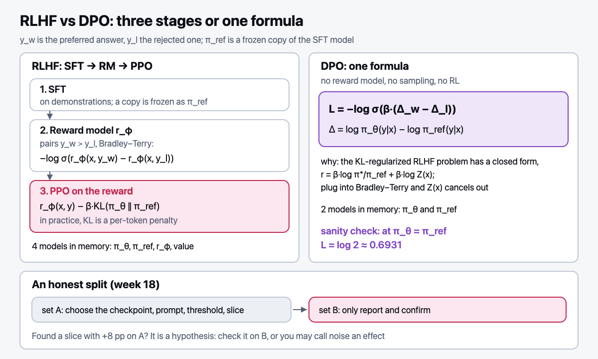
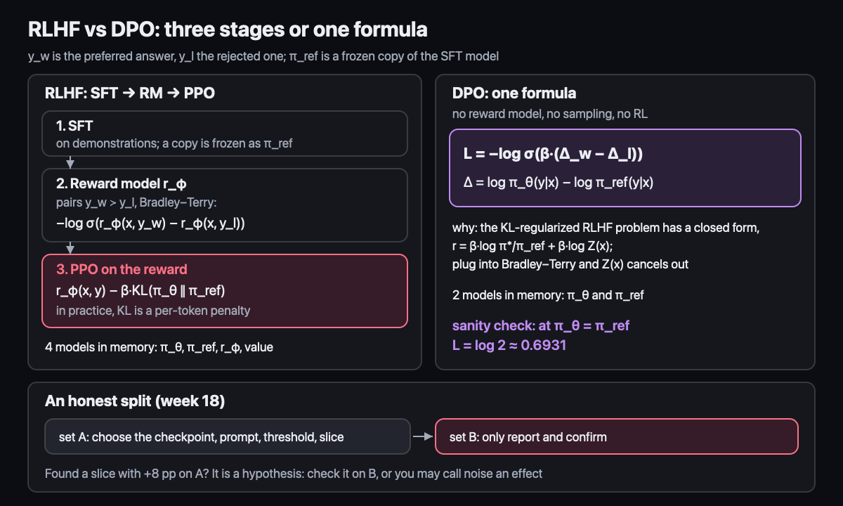
• Reward model (a model that outputs a scalar score for an answer), the Bradley–Terry model (probability of preference σ(r_A − r_B)). Notice that its loss is really ordinary binary cross-entropy with a label that is always 1
• The full RLHF pipeline: SFT → RM → PPO. The KL penalty to the reference model (a frozen copy of the SFT model) in practice folds into a per-token reward
• Reward hacking (the policy gets a high reward without doing what was intended: for example, it writes long answers because the RM likes length)

Where the formula itself comes from. Bradley–Terry (1952) grows out of random utility models. In Thurstone (1927), a person does not compare r_A and r_B but noisy r_A + ε_A and r_B + ε_B, and picks the larger one. Normal noise gives the probit Φ((r_A − r_B)/(σ√2)). Gumbel noise (the distribution of a maximum) gives a logistic difference of noises and exactly σ(r_A − r_B); Luce's choice axiom (1959) leads to the same place, and for a choice among many answers you get softmax. Consequence: the reward is defined only up to a shift, since r + c gives the same probabilities. Only differences of RM scores carry meaning.

When preferences do not fit into a single number. One number per answer is possible only if preferences are complete (any two answers are comparable) and transitive (A ≻ B and B ≻ C imply A ≻ C). In plain terms. Three answers. Annotators pick A over B 70% of the time, B over C 70%, and C over A also 70%: a cycle A ≻ B ≻ C ≻ A. This happens when people compare on different criteria: one on brevity, another on accuracy. Each pair asks for a difference of ln(0.7/0.3) ≈ 0.85, but three differences around the cycle must sum to 0, not 2.54. The best that numbers can do: r_A = r_B = r_C, a prediction of 0.5 in every pair, a loss of ln 2 ≈ 0.693 per pair. The lower bound for any model is the entropy of the labels, −(0.7·ln 0.7 + 0.3·ln 0.3) ≈ 0.611. The gap of 0.082 nats per pair cannot be closed by any RM architecture: it is baked into the "one number per answer" setup. Why the minimum is at equal rewards: the pair loss is convex in the difference, the mean of the three differences is 0, so by Jensen's inequality the sum of losses is at least three times the value at zero. With a cycle there is no "best" answer at all: against the mixture (⅓, ⅓, ⅓) each answer wins exactly half of the comparisons.

The Condorcet cycle and Arrow's theorem. Such a cycle has a name: the Condorcet cycle (or paradox). It appears even when each annotator on their own reasons consistently. Three annotators: the first ranks A ≻ B ≻ C, the second B ≻ C ≻ A, the third C ≻ A ≻ B. In every pair the score is 2:1, and the majority view goes around the circle A ≻ B ≻ C ≻ A. Arrow's theorem (1951) says this is not the fault of an unlucky voting rule: with three or more options there is no way to turn the rankings of many people into one common ranking that at the same time (1) works for any tastes, (2) puts A above B whenever everyone does, (3) settles A versus B only by how people compared A and B themselves, and (4) does not reduce to the taste of a single person (a "dictator"). The takeaway for RLHF: a reward model learns from the comparisons of many annotators and must produce one scale, so it averages incompatible tastes. The policy then optimizes the taste of an "average annotator" who may not exist among real people, and a minority with a different taste dissolves in the average. More: MIT OCW 6.254, lecture 21 on social choice (link also in Resources).

Reward hacking through an economist's eyes. Economists would call this a principal-agent problem. The principal (the developer) wants quality but sees only a proxy (a stand-in for the goal): the RM score. The agent (the policy) is paid for the proxy, and when incentives diverge you get moral hazard: the agent does what it is paid for, not what is needed. Goodhart's law (1975) says the same: a measure that becomes a target stops being a good measure. The tools of contract theory (Holmström, 1979) are instantly recognizable: do not let the agent stray far from verified behavior (KL penalty to the reference), pay for a verifiable result (RLVR), use several independent signals instead of one, and manually inspect a sample of answers. This is an analogy for intuition, not a theory of how RLHF works.

In plain terms. For one prompt you sample 4 answers, and the verifier assigns rewards (1, 0, 0, 1). The baseline is the group mean, 0.5; advantages are (+0.5, −0.5, −0.5, +0.5), and after dividing by the std of 0.5 you get ±1. No value model is needed: the mean is measured, not predicted. Two failure modes show up on the same numbers. The group (1, 1, 1, 0) is almost fully solved, but its std is 0.43, and the wrong answer gets −1.73: larger in magnitude than any answer in an informative group. If the advantage is divided by answer length, a wrong 16-token answer gets −1/16 per token, while a 2-token one gets −1/2: the long mistake is punished 8 times more weakly.

• GRPO (Group Relative Policy Optimization) = three known ideas combined: the off-policy surrogate (step 3) + PPO clipping (step 4)
  • group normalization of the advantage. After week 16 this is not a new construction. No value head is needed: the baseline is not learned but measured by sampling. More compute (G generations per prompt), less memory
• Dr. GRPO: two specific failure modes of GRPO. Dividing by std(r) inflates the gradient on degenerately easy and hard groups. Normalizing by answer length means that among wrong answers, long ones are penalized more weakly. The model learns that if you do not know the answer, you should write a lot
• Degenerate groups and problems at the edge of capability. In plain terms. The model solves a problem with probability p, and a group has G = 4 answers. If all 4 are right or all are wrong, the advantages are zero and there is no gradient. At p = 0.5 this happens in 12.5% of groups, at p = 0.9 already in 66%, at p = 0.97 in 89%. Formula: the share of empty groups is p^G + (1 − p)^G, and the reward variance p(1 − p) peaks at p = 0.5. As the model learns, a fixed set of problems becomes easy: the signal fades. So problems are chosen to keep p in the middle: degenerate groups are dropped and new ones are sampled, or problems are generated by a program with adjustable difficulty, and the difficulty follows the model (Faro et al., Frontier Learning, 2026). A larger G also helps: at p = 0.9 and G = 16 empty groups are 19%

In plain terms. One pair: the chosen answer y_w and the rejected y_l, β = 0.1. At the start π_θ = π_ref, the difference of log-ratios is 0, and the loss is −log σ(0) = log 2 ≈ 0.693. This is a check value; you will need it below. After training, log π_θ(y_w) has risen by 2 relative to the reference, and log π_θ(y_l) has dropped by 3. The margin is β·(2 − (−3)) = 0.5, and the loss is −log σ(0.5) ≈ 0.474. You get the same loss if both answers drop: the chosen by 1, the rejected by 6. DPO only looks at the difference. That is why under DPO the probability of the chosen answer can go down too.

• DPO: derive it from the RLHF objective. The KL-regularized problem has a closed-form solution; express the reward through the ratio of policies and plug it into Bradley–Terry → a loss with no reward model and no RL at all
• Comparing PPO / GRPO / DPO / RLAIF (a model labels the preferences, not a human): when to use which

• RLVR (RL with verifiable rewards: a program checks the answer), reasoning models, test-time compute (more compute at answer time: long reasoning, several attempts; covered in detail in week 18, subsection "Test-time compute")

Reward functions for RLVR

RLVR (RL with verifiable rewards) replaces the reward model with a checker program that compares the answer with a reference. Length and a confident tone cannot bribe a program, but a person writes it, and the policy will find every hole in it: reward hacking has not gone away, it has moved into the checker's code.

In plain terms. A GSM8K-style problem (grade-school arithmetic word problems): "3 boxes of 4 apples, 2 apples were eaten. How many are left?", reference answer 10. The model is trained to write its reasoning and put the result after the marker ####. The reward has two parts: 1 for the right number after the marker and 0.1 for format (exactly one marker, followed by a number).

The third answer is right in substance, but the checker does not see the number. A partial reward, say 0.5 for the right number anywhere in the text, would give it 0.5. But then the answer "1 2 3 … 100" gets 0.5 on every problem: listing all the numbers is cheaper than solving.

• Why a format-only reward leads to hacking. If you pay only for #### number, the answer #### 7 with no reasoning at all gets the maximum. The policy quickly learns the format, and every answer in a group gets the same 0.1: the signal disappears, and correctness does not move. A format bonus helps as a hint at the start, and only when it is small compared with correctness (0.1 versus 1): then a right answer always beats a pretty one
• Empty groups. If all G answers get the same reward (all 1.1 or all 0), group_advantages from nanolm/rl.py subtracts the mean and gets zeros; dividing by std + eps leaves them zero. The gradient from such a group is exactly zero, even though compute was spent generating it. Log the share of empty groups (above: p^G + (1 − p)^G) at every step. A format bonus and a partial reward break ties: the group (0, 0.1, 0, 0) already gives a gradient, but it teaches format, not solving
• A partial reward is needed when the full one is almost always 0 (hard problems, a small model): otherwise almost every group is empty. Every such loophole gets checked for hacking: read the 20 highest-reward answers by eye
• A practical rule of thumb. Models below roughly 1.5B parameters rarely start to reason under RLVR: the base model almost never solves the problem, the reward is almost always 0, the groups are empty, there is nothing to learn from. The mean reward does not grow right away: for the first tens or hundreds of steps the curve is nearly flat, the model masters the format first, and only then correctness rises. Stopping a run because the start of the curve is flat is a common mistake

One GRPO step end to end

The GRPO formulas above are written in terms of answer log-probabilities. This part is about how to compute them and in what order the pieces of one step go: this seam is where code that looks correct most often breaks.

In plain terms. The prompt "2 + 2 =", an answer of three tokens. The model gave the actual answer tokens probabilities 0.5, 0.25 and 0.8. By the chain rule (the probability of a sequence is the product of the conditional probabilities of its tokens) the probability of the answer is 0.5 · 0.25 · 0.8 = 0.1, and its log is the sum ln 0.5 + ln 0.25 + ln 0.8 = −0.69 − 1.39 − 0.22 = −2.30 = ln 0.1. The mean −0.77 gives e^{−0.77} ≈ 0.46: that is the geometric mean of the token probabilities, not the probability of the answer. Prompt tokens are not part of the sum, since the model did not write them. Padding (filler tokens that bring shorter answers up to the common length T) is not part of it either. Shift by one: the model output at position t predicts token t + 1, so the probability 0.5 of the first answer token comes from the output at the last prompt token.

• Sum or mean. The probability ratio of a whole answer is exp(Σ log π_θ − Σ log π_old) over the answer tokens, and that needs the sum. Taking the mean instead means dividing by the answer length, which is exactly the GRPO normalization 1/|o| that Dr. GRPO calls a bias (above: a long mistake is punished less). nanolm/rl.py makes this choice explicit: grpo_loss averages inside each answer (sequence_masked_mean), dr_grpo_loss divides by the total number of tokens (masked_mean). Make the choice on purpose, not because .mean() is shorter. You can compute an answer log-probability with the shift and the mask in the trainer task sequence_logprob
• Simplified GRPO without KL (β = 0). Many RLVR recipes (Dr. GRPO, DAPO) drop the KL penalty to the reference model. A checker cannot be bribed by smooth text the way a reward model can, so the main reason to stay near the reference is weaker. The reference costs another copy of the weights in memory and another forward pass at every step. KL also pulls back the long reasoning that the whole exercise is for. KL comes back when a learned reward model gives the reward (it gets hacked), when the language degrades (answers mix languages, loop) and when many epochs run over a small problem set. Without KL the only guard against drifting away is clipping, and only within one batch (week 16)

The order of one step on B prompts, with the functions from nanolm/rl.py:

1. Sample G answers to each prompt with the current policy at a temperature above 0: with greedy decoding all G answers coincide, and the group is empty in advance. The model is in eval() mode, without gradients.
2. Score the answers with the checker (the trainer task rlvr_reward) and log the share of empty groups.
3. Group advantages: group_advantages, rewards of shape (B, G).
4. Old log-probabilities old_logprobs: a pass of the same model under torch.no_grad() and in eval(). With β > 0, compute ref_logprobs the same way with the frozen reference model.
5. New log-probabilities with gradients: sequence_logprobs (per token, shape (B·G, T)) and the answer mask.
6. Loss: grpo_loss or dr_grpo_loss; with β > 0 add β · kl_penalty_k3(logprobs, ref_logprobs, mask).
7. backward, gradient norm clipping, an optimizer step. If several steps are taken on the same rollouts, old_logprobs are not recomputed: they are what defines π_old.

With one step per batch the ratio π_θ/π_old is identically 1, clipping never fires, and GRPO reduces to REINFORCE with a group baseline (this is what test_surrogate_reduces_to_reinforce_at_theta_old from week 16 checks). π_old and clipping are needed only when several steps are taken on the same rollouts.

Where the step breaks

• The model mode bug. Generation and old_logprobs are computed in train() mode. Dropout (randomly zeroing part of the activations during training) silences different neurons on every pass, and two passes with identical weights give different log-probabilities. On the first step the ratio π_θ/π_old must be exactly 1, but it comes out as 0.9 on one token and 1.15 on another: clipping cuts the gradient where the policy has not moved at all. model.eval() turns dropout off but still builds the computation graph; torch.no_grad() builds no graph but leaves dropout alone. These are two separate switches, and both are needed. In RL fine-tuning dropout is usually turned off in the gradient pass too (modern LLMs barely use it anyway, week 8). A one-line check: on the first step max |ratio − 1| is at the level of rounding error. The same symptom appears when a separate inference engine generates in a different precision: then old_logprobs are recomputed with the trained model instead of taken from the generator
• old_logprobs with gradients. The old log-probabilities were computed with the same weights without no_grad and without .detach(). Then the ratio exp(log π_θ − log π_old) depends on θ through both the numerator and the denominator, and its derivative is zero: the loss is computed, but the gradient is exactly zero. The graph also takes twice the memory
• Mask and shift. Prompt and padding log-probabilities got into the sum, or the mask was not shifted together with the target tokens and the first answer token was lost. A comparison with a loop on a small example catches it

Practice on a real model (optional). The GRPO notebook from Unsloth (link in Resources, the Post-training section) runs in free Colab on a T4: LoRA (week 15) on top of a model of 1.5B parameters and up, GSM8K-style problems. What to measure: the correctness reward and the format reward separately at every step; the share of empty groups; the mean answer length; the 20 highest-reward answers (any hacking?). Compare two runs: one with a format-only reward and one with the full reward. In the first, format quickly reaches 100% while accuracy on held-out problems stays flat. You can write the reward function and the share of empty groups yourself in the trainer task rlvr_reward.

A second path: GRPO from scratch on MATH (optional). Sebastian Raschka's book Build a Reasoning Model (From Scratch) (chapter 6, code in the reasoning-from-scratch repository) and episode 6 of his companion video series build RLVR and GRPO in PyTorch without RL libraries, on MATH problems (competition-level problems whose answer a program checks). Links are in Resources, the Post-training section. Check the GRPO step there against the subsection "One GRPO step end to end". What to measure: accuracy on MATH-500 (500 problems from the MATH test split, the usual subset for quick measurements) before training and every few dozen steps; mean answer length separately for correct and wrong answers (growing length of wrong answers reveals the length normalization bias); the share of empty groups; peak GPU memory at different G and maximum answer lengths. Memory grows roughly in proportion to B · G · T (activations of the gradient pass), and with β > 0 the reference model is added on top.

Code → nanolm/rl.py: group_advantages, grpo_loss, dr_grpo_loss, kl_penalty_k3, dpo_loss, bradley_terry_loss.

DPO check: at π_θ = π_ref the loss must be exactly log 2 ≈ 0.6931. Got something else? There is no point going further; find the bug.

scripts/rl_demo.py shows both GRPO biases in numbers: a degenerate group gets a larger advantage than an informative one, and an answer of length 16 gets a per-token gradient 8 times smaller than an answer of length 2.

Math (Track D): D25: the closed-form solution of the KL-regularized problem; D26: Bradley–Terry and the DPO loss.

Interview question of the week: "What is the difference between PPO and GRPO?" This question gets asked word for word. Give a 3-minute answer with formulas. After week 16 it should sound like "both are built on the same surrogate and differ only in the baseline".

Sources: Ouyang et al., InstructGPT (2022); Rafailov et al., DPO (2023); Shao et al., DeepSeekMath (2024), which introduced GRPO; Liu et al., Understanding R1-Zero-Like Training, Dr. GRPO (2025); Faro et al., Frontier Learning (2026), problems at the edge of capability; Cobbe et al., GSM8K (2021); Hendrycks et al., MATH (2021); Lightman et al., Let's Verify Step by Step (2023), the MATH-500 subset; Yu et al., DAPO (2025); Raschka, Build a Reasoning Model (From Scratch), chapter 6 (practice, links in Resources).

Deeper: 05-ГЛУБИНА, sections "★★ Weeks 16–17. The missing link between REINFORCE and PPO" and "Weeks 17 and 21. A little game theory".

Week outcomes

• I can derive the DPO loss from the KL-regularized RLHF objective.
• I can answer "PPO vs GRPO" in 3 minutes with formulas.
• I can explain the two GRPO failure modes that Dr. GRPO fixes, with numbers from rl_demo.py.
• I can implement dpo_loss and check the value log 2 at π_θ = π_ref.
• I can explain the Condorcet cycle and Arrow's theorem with the three-annotator example and what they imply for a single reward model.
• I can lay out one GRPO step from sampling to the optimizer step and say where eval(), no_grad and the answer mask are needed.

Self-check

1. Why does the Bradley–Terry loss turn out to be binary cross-entropy with label 1?
2. What is reward hacking? Give an example and a defense.
3. When would you choose DPO, and when GRPO?
4. The labels form a cycle A ≻ B ≻ C ≻ A at 70% each. What is the best Bradley–Terry loss, and why can it not be pushed down to the entropy of the labels?
5. Why does GRPO stop learning on a problem set the model has almost solved? Compute the share of empty groups at p = 0.9, G = 8.
6. Why does a format-only reward lead to reward hacking, while a 0.1 format bonus together with a reward of 1 for correctness helps?
7. All 8 answers in a group got reward 0. What does group_advantages return, and what gradient does the group give? What changes if two of the eight get the format bonus?
8. Why does RLVR on a model below roughly 1.5B parameters often fail to teach reasoning even though the code is correct? Which logged metric shows it?
9. Three annotators with consistent tastes produce the majority cycle A ≻ B ≻ C ≻ A. What is this phenomenon called, what does Arrow's theorem state, and what does it mean for a single reward model?
10. An answer of four tokens got probabilities 0.5, 0.5, 0.8 and 0.5. What is its log-probability, which positions does the mask exclude, and how is the model output shifted relative to the tokens? What changes in GRPO if you take the mean instead of the sum?
11. On the first GRPO step the ratio π_θ/π_old is 0.9 and 1.15 on some tokens, although the weights have not been updated yet. Which mode bug causes this, and what check catches it? What happens to the gradient if old_logprobs are computed without no_grad?